Probability CheatSheet
Overview
Teaching: min
Exercises: minQuestions
Counting
Multiplication Rule
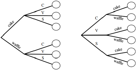
Let’s say we have a compound experiment (an experiment with multiple components). If the 1st component has \(n_1\) possible outcomes, the 2nd component has \(n_2\) possible outcomes, …, and the \(r\)th component has \(n_r\) possible outcomes, then overall there are \(n_1n_2 \dots n_r\) possibilities for the whole experiment.
Sampling Table
The sampling table gives the number of possible samples of size \(k\) out of a population of size \(n\), under various assumptions about how the sample is collected.
| Order Matters | Not Matter | |
|---|---|---|
| With Replacement | \(n^k\) | \({n+k-1 \choose k}\) |
| Without Replacement | \(\frac{n!}{(n - k)!}\) | \({n \choose k}\) |
Naive Definition of Probability
If all outcomes are equally likely, the probability of an event \(A\) happening is:
[P_{\textrm{naive}}(A) = \frac{\text{number of outcomes favorable to $A$}}{\text{number of outcomes}}]
Independence
Independent Events:
\(A\) and \(B\) are independent if knowing whether \(A\) occurred gives no information about whether \(B\) occurred. More formally, \(A\) and \(B\) (which have nonzero probability) are independent if and only if one of the following equivalent statements holds:
֍ \(P(A \cap B) = P(A)P(B)\)
֍ \(P(A|B) = P(A)\)
֍ \(P(B|A) = P(B)\)
Conditional Independence:
\(A\) and \(B\) are conditionally independent given \(C\) if
\(P(A \cap B\|C) = P(A\|C)P(B\|C)\).
Conditional independence does not imply independence, and independence does not imply conditional independence.
Unions, Intersections, and Complements
֍ De Morgan’s Laws: A useful identity that can make calculating probabilities of unions easier by relating them to intersections, and vice versa. Analogous results hold with more than two sets.
֍ \((A \cup B)^c = A^c \cap B^c\)
֍ \((A \cap B)^c = A^c \cup B^c\)
Joint, Marginal, and Conditional
֍ Joint Probability: \(P(A \cap B)\) or \(P(A, B)\) – Probability of \(A\) and \(B\).
֍ Marginal (Unconditional) Probability: \(P(A)\) – Probability of \(A\).
֍ Conditional Probability: \(P(A\|B) = \frac{P(A, B)}{P(B)}\) – Probability of \(A\), given that \(B\) occurred.
֍ Conditional Probability is Probability: \(P(A\|B)\) is a probability function for any fixed \(B\). Any theorem that holds for probability also holds for conditional probability.
Probability of an Intersection or Union
Intersections via Conditioning
[\begin{align}
P(A,B) &= P(A)P(B|A)
P(A,B,C) &= P(A)P(B|A)P(C|A,B)
\end{align}]
Unions via Inclusion-Exclusion
[\begin{align}
P(A \cup B) &= P(A) + P(B) - P(A \cap B)
P(A \cup B \cup C) &= P(A) + P(B) + P(C)
&\quad - P(A \cap B) - P(A \cap C) - P(B \cap C)
&\quad + P(A \cap B \cap C)
\end{align}]
Simpson’s Paradox
It is possible to have \(P(A\mid B,C) < P(A\mid B^c, C) \text{ and } P(A\mid B, C^c) < P(A \mid B^c, C^c)\) \(\text{yet also } P(A\mid B) > P(A \mid B^c).\)
Law of Total Probability (LOTP)
Let \({ B}_1, { B}_2, { B}_3, ... { B}_n\) be a partition of the sample space (i.e., they are disjoint and their union is the entire sample space).
[\begin{align}
P({ A}) &= P({ A} | { B}_1)P({ B}_1) + P({ A} | { B}_2)P({ B}_2) + \dots + P({ A} | { B}_n)P({ B}_n)
P({ A}) &= P({ A} \cap { B}_1)+ P({ A} \cap { B}_2)+ \dots + P({ A} \cap { B}_n)
\end{align}]
For LOTP with extra conditioning, just add in another event \(C\)!
[\begin{align}
P({ A}| { C}) &= P({ A} | { B}_1, { C})P({ B}_1 | { C}) + \dots + P({ A} | { B}_n, { C})P({ B}_n | { C})
P({ A}| { C}) &= P({ A} \cap { B}_1 | { C})+ P({ A} \cap { B}_2 | { C})+ \dots + P({ A} \cap { B}_n | { C})
\end{align}]
Special case of LOTP with \({ B}\) and \({ B^c}\) as partition:
[\begin{align}
P({ A}) &= P({ A} | { B})P({ B}) + P({ A} | { B^c})P({ B^c})
P({ A}) &= P({ A} \cap { B})+ P({ A} \cap { B^c})
\end{align}]
Bayes’ Rule
Bayes’ Rule, with extra conditioning (just add in \(C\)!)
| [P({ A} | { B}) = \frac{P({ B} | { A})P({ A})}{P({ B})}] |
| [P({ A} | { B}, { C}) = \frac{P({ B} | { A}, { C})P({ A} | { C})}{P({ B} | { C})}] |
We can also write
| [P(A | B,C) = \frac{P(A,B,C)}{P(B,C)} = \frac{P(B,C | A)P(A)}{P(B,C)}] |
Odds Form of Bayes’ Rule
\(\frac{P({ A}\| { B})}{P({ A^c}\| { B})} = \frac{P({ B}\|{ A})}{P({ B}| { A^c})}\frac{P({ A})}{P({ A^c})}\)
The posterior odds of \(A\) are the likelihood ratio times the prior odds.
Random Variables and their Distributions
PMF, CDF, and Independence
Probability Mass Function (PMF)
Gives the probability that a discrete random variable takes on the value x.
[p_X(x) = P(X=x)]
The PMF satisfies:
\(p_X(x) \geq 0 \quad \textrm{and} \quad \sum_x p_X(x) = 1\)
Cumulative Distribution Function (CDF)
Gives the probability that a random variable is less than or equal to x.
[F_X(x) = P(X \leq x)]
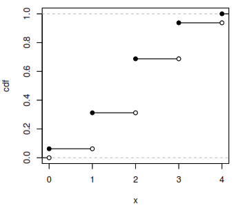
The CDF is an increasing, right-continuous function with:
\(F_X(x) \to 0 \quad \textrm{as} \quad x \to -\infty \quad \textrm{and} \quad F_X(x) \to 1 \quad \textrm{as} \quad x \to \infty\)
Independence
Intuitively, two random variables are independent if knowing the value of one gives no information about the other. Discrete random variables X and Y are independent if for all values of x and y:
[P(X=x, Y=y) = P(X = x)P(Y = y)]
Expected Value and Indicators
Expected Value and Linearity
Expected Value
(a.k.a. mean, expectation, or average) is a weighted average of the possible outcomes of our random variable.
Mathematically, if x1, x2, x3, … are all of the distinct possible values that X can take, the expected value of X is:
\(E(X) = \sum\limits_{i}x_iP(X=x_i)\)
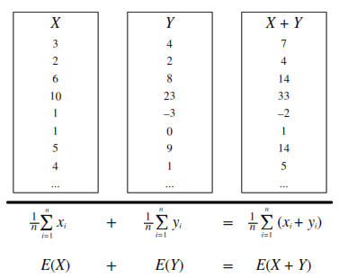 Linearity
For any random variables X and Y, and constants a, b, c:
[E(aX + bY + c) = aE(X) + bE(Y) + c]
Same distribution implies same mean
If X and Y have the same distribution, then E(X) = E(Y) and, more generally:
[E(g(X)) = E(g(Y))]
Conditional Expected Value
Conditional expected value is defined like expectation, only conditioned on any event A:
| [E(X | A) = \sum\limits_{x}xP(X=x | A)] |
Indicator Random Variables
Indicator Random Variable An indicator random variable is a random variable that takes on the value 1 or 0. It is always an indicator of some event: if the event occurs, the indicator is 1; otherwise, it is 0. They are useful for many problems about counting how many events of some kind occur. Write:
[I_A =
\begin{cases}
1 & \text{if $A$ occurs},
0 & \text{if $A$ does not occur}.
\end{cases}]
Note that: \(I_A^2 = I_A\), \(I_A I_B = I_{A \cap B}\), \(I_{A \cup B} = I_A + I_B - I_A I_B\)
Distribution
\(I_A \sim Bern(p) where p = P(A)\).
Fundamental Bridge
The expectation of the indicator for event A is the probability of event A: \(E(I_A) = P(A)\).
Variance and Standard Deviation
[var(X) = E \left(X - E(X)\right)^2 = E(X^2) - (E(X))^2]
[\textrm{SD}(X) = \sqrt{var(X)}]
Continuous RVs, LOTUS, UoU
Continuous Random Variables (CRVs)
What is a Continuous Random Variable (CRV)?
A continuous random variable can take on any possible value within a certain interval (for example, [0, 1]), whereas a discrete random variable can only take on variables in a list of countable values (for example, all the integers, or the values 1, 1/2, 1/4, 1/8, etc.)
Do Continuous Random Variables have PMFs?
No. The probability that a continuous random variable takes on any specific value is 0.
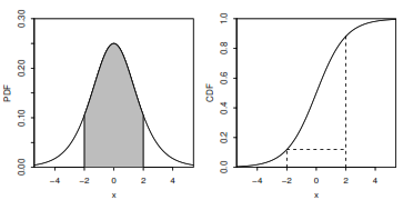
What’s the probability that a CRV is in an interval?
Take the difference in CDF values (or use the PDF as described later).
[P(a \leq X \leq b) = P(X \leq b) - P(X \leq a) = F_X(b) - F_X(a)]
For X ~ N(μ, σ^2), this becomes
[P(a \leq X \leq b) = \Phi\left(\frac{b-\mu}{\sigma}\right) - \Phi\left(\frac{a-\mu}{\sigma}\right)]
What is the Probability Density Function (PDF)?
The PDF f is the derivative of the CDF F.
[F’(x) = f(x)]
A PDF is nonnegative and integrates to 1. By the fundamental theorem of calculus, to get from PDF back to CDF we can integrate:
\(F(x) = \int_{-\infty}^x f(t)dt\)
To find the probability that a CRV takes on a value in an interval, integrate the PDF over that interval.
[F(b) - F(a) = \int_a^b f(x)dx]
How do I find the expected value of a CRV?
Analogous to the discrete case, where you sum x times the PMF, for CRVs you integrate x times the PDF.
[E(X) = \int_{-\infty}^\infty xf(x)dx]
LOTUS
Expected value of a function of an r.v.
The expected value of X is defined this way:
\(E(X) = \sum_x xP(X=x) \text{ (for discrete X)}\) \(E(X) = \int_{-\infty}^\infty xf(x)dx \text{ (for continuous X)}\)
The Law of the Unconscious Statistician (LOTUS) states that you can find the expected value of a function of a random variable, g(X), in a similar way, by replacing the x in front of the PMF/PDF by g(x) but still working with the PMF/PDF of X:
\(E(g(X)) = \sum_x g(x)P(X=x) \text{ (for discrete X)}\) \(E(g(X)) = \int_{-\infty}^\infty g(x)f(x)dx \text{ (for continuous X)}\)
What’s a function of a random variable?
A function of a random variable is also a random variable. For example, if X is the number of bikes you see in an hour, then g(X) = 2X is the number of bike wheels you see in that hour, and h(X) = \({X \choose 2} = \frac{X(X-1)}{2}\) is the number of pairs of bikes such that you see both of those bikes in that hour.
What’s the point?
You don’t need to know the PMF/PDF of g(X) to find its expected value. All you need is the PMF/PDF of X.
Universality of Uniform (UoU)
When you plug any CRV into its own CDF, you get a Uniform(0,1) random variable. When you plug a Uniform(0,1) r.v. into an inverse CDF, you get an r.v. with that CDF. For example, let’s say that a random variable X has CDF
[F(x) = 1 - e^{-x}, \textrm{ for } x>0]
By UoU, if we plug X into this function then we get a uniformly distributed random variable.
[F(X) = 1 - e^{-X} \sim \textrm{Unif}(0,1)]
Similarly, if \(U ~ Unif(0,1)\) then \(F^{-1}(U)\) has CDF \(F\). The key point is that for any continuous random variable \(X\), we can transform it into a Uniform random variable and back by using its CDF.
Moments
Moments describe the shape of a distribution. Let X have mean μ and standard deviation σ, and Z=(X-μ)/σ be the standardized version of X. The kth moment of X is μₖ = E(Xᵏ), and the kth standardized moment of X is mₖ = E(Zᵏ). The mean, variance, skewness, and kurtosis are important summaries of the shape of a distribution.
֍ Mean: \(E(X) = μ₁\)
֍ Variance: \(var(X) = μ₂ - μ₁²\)
֍ Skewness: \(skew(X) = m₃\)
֍ Kurtosis: \(kurt(X) = m₄ - 3\)
Moment Generating Functions
- MGF (Moment Generating Function): For any random variable X, the function
\(Mₓ(t) = E(e^{tX})\)
is the moment generating function (MGF) of X, if it exists for all t in some open interval containing 0. The variable t could just as well have been called u or v. It’s a bookkeeping device that lets us work with the function Mₓ rather than the sequence of moments. - Why is it called the Moment Generating Function? Because the kth derivative of the moment generating function, evaluated at 0, is the kth moment of X.
\(μₖ = E(Xᵏ) = Mₓ⁽ᵏ⁾(0)\)
This is true by Taylor expansion of \(e^{tX}\) since
\(Mₓ(t) = E(e^{tX}) = ∑_(k=0)^(∞) [\frac{E(Xᵏ)tᵏ}{k!}] = ∑_(k=0)^(∞) [\frac{μₖtᵏ}{k!}]\) - MGF of linear functions: If \(Y = aX + b\), then \(Mₙ(t) = E(e^(t(aX + b))) = e^(bt)Mₓ(at)\)
- Uniqueness: If it exists, the MGF uniquely determines the distribution. This means that for any two random variables X and Y, they are distributed the same (their PMFs/PDFs are equal) if and only if their MGFs are equal.
- Summing Independent RVs by Multiplying MGFs: If X and Y are independent, then
\(Mₓ₊ᵧ(t) = E(e^(t(X + Y))) = E(e^{tX})E(e^(tY)) = Mₓ(t) ⋅ Mᵧ(t)\)
The MGF of the sum of two random variables is the product of the MGFs of those two random variables.
Joint PDFs and CDFs
Joint Distributions
- Joint CDF: The joint cumulative distribution function (CDF) of X and Y is \(F(x,y) = P(X ≤ x, Y ≤ y)\).
- Joint PMF: In the discrete case, X and Y have a joint probability mass function \((PMF)\)
\(pₓᵧ(x,y) = P(X=x, Y=y)\). - Joint PDF: In the continuous case, X and Y have a joint probability density function \((PDF)\)
\(fₓᵧ(x,y) = (∂²/∂x∂y)Fₓᵧ(x,y)\).
The joint PMF/PDF must be nonnegative and sum/integrate to 1.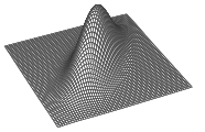
Conditional Distributions
֍ Conditioning and Bayes’ rule for discrete random variables:
\(P(Y=y|X=x) = P(X=x,Y=y) / P(X=x)\)
\(= P(X=x|Y=y)P(Y=y) / ∑ᵧ P(X=x|Y=ᵧ)P(Y=ᵧ)\)
֍ Conditioning and Bayes’ rule for continuous random variables:
\(fᵧ|ₓ(y|x) = fₓᵧ(x, y) / fₓ(x)\)
\(= (fₓ|ᵧ(x|y)fᵧ(y)) / fₓ(x)\)
֍ Hybrid Bayes’ rule:
\(fₓ(x|A) = (P(A | X = x)fₓ(x)) / P(A)\)
Marginal Distributions
To find the distribution of one (or more) random variables from a joint PMF/PDF, sum/integrate over the unwanted random variables.\
֍ Marginal PMF from joint PMF:
\(P(X = x) = ∑ₓ P(X=x, Y=y)\)
֍ Marginal PDF from joint PDF:
\(fₓ(x) = ∫[∞, -∞] fₓᵧ(x, y) dy\)
Independence of Random Variables
Random variables X and Y are independent if and only if any of the following conditions holds:
֍ Joint CDF is the product of the marginal CDFs.
֍ Joint PMF/PDF is the product of the marginal PMFs/PDFs.
֍ Conditional distribution of Y given X is the marginal distribution of Y.
Write X ⫫ Y to denote that X and Y are independent.
Multivariate LOTUS
Law of the unconscious statistician (LOTUS) in more than one dimension is analogous to the 1D LOTUS.
For discrete random variables:
\(E(g(X, Y)) = ∑ₓ∑y g(x, y)P(X=x, Y=y)\)
For continuous random variables:
\(E(g(X, Y)) = ∫[-∞, ∞]∫[-∞, ∞] g(x, y)fₓᵧ(x, y)dxdy\)
Covariance and Transformations
Covariance and Correlation
Covariance is the analog of variance for two random variables. \(\text{cov}(X, Y) = E\left((X - E(X))(Y - E(Y))\right) = E(XY) - E(X)E(Y)\) Note that \(\text{cov}(X, X) = E(X^2) - (E(X))^2 = \text{var}(X)\)
Correlation is a standardized version of covariance that is always between \(-1\) and \(1\). \(\text{corr}(X, Y) = \frac{\text{cov}(X, Y)}{\sqrt{\text{var}(X)\text{var}(Y)}}\)
Covariance and Independence If two random variables are independent, then they are uncorrelated. The converse is not necessarily true (e.g., consider \(X \sim \mathcal{N}(0,1)\) and \(Y=X^2\)).
\(X \perp Y \longrightarrow \text{cov}(X, Y) = 0 \longrightarrow E(XY) = E(X)E(Y)\)
Covariance and Variance The variance of a sum can be found by \(var(X + Y) = var(X) + var(Y) + 2\text{cov}(X, Y)\) \(var(X_1 + X_2 + \dots + X_n ) = \sum_{i = 1}^{n}var(X_i) + 2\sum_{i < j} \text{cov}(X_i, X_j)\) If \(X\) and \(Y\) are independent, then they have covariance \(0\), so \(X \perp Y \Longrightarrow var(X + Y) = var(X) + var(Y)\) If \(X_1, X_2, \dots, X_n\) are identically distributed and have the same covariance relationships (often by symmetry), then \(var(X_1 + X_2 + \dots + X_n ) = nvar(X_1) + 2{n \choose 2}\text{cov}(X_1, X_2)\)
Covariance Properties For random variables \(W, X, Y, Z\) and constants \(a, b\): \(\text{cov}(X, Y) = \text{cov}(Y, X)\) \(\text{cov}(X + a, Y + b) = \text{cov}(X, Y)\) \(\text{cov}(aX, bY) = ab\text{cov}(X, Y)\) \(\text{cov}(W + X, Y + Z) = \text{cov}(W, Y) + \text{cov}(W, Z) + \text{cov}(X, Y) + \text{cov}(X, Z)\)
Correlation is location-invariant and scale-invariant For any constants \(a,b,c,d\) with \(a\) and \(c\) nonzero, \(\text{corr}(aX + b, cY + d) = \text{corr}(X, Y)\)
Transformations
One Variable Transformations Let’s say that we have a random variable \(X\) with PDF \(f_X(x)\), but we are also interested in some function of \(X\). We call this function \(Y = g(X)\). Also let \(y=g(x)\). If \(g\) is differentiable and strictly increasing (or strictly decreasing), then the PDF of \(Y\) is \(f_Y(y) = f_X(x)\left|\frac{dx}{dy}\right| = f_X(g^{-1}(y))\left|\frac{d}{dy}g^{-1}(y)\right|\) The derivative of the inverse transformation is called the Jacobian.
Two Variable Transformations Similarly, let’s say we know the joint PDF of \(U\) and \(V\) but are also interested in the random vector \((X, Y)\) defined by \((X, Y) = g(U, V)\). Let \(\frac{\partial (u,v)}{\partial (x,y)} = \begin{pmatrix} \frac{\partial u}{\partial x} & \frac{\partial u}{\partial y} \\ \frac{\partial v}{\partial x} & \frac{\partial v}{\partial y} \\ \end{pmatrix}\) be the Jacobian matrix. If the entries in this matrix exist and are continuous, and the determinant of the matrix is never \(0\), then \(f_{X,Y}(x, y) = f_{U,V}(u,v) \left|\left| \frac{\partial (u,v)}{\partial (x,y)}\right| \right|\) The inner bars tell us to take the matrix’s determinant, and the outer bars tell us to take the absolute value. In a \(2 \times 2\) matrix, \(\left| \left| \begin{array}{ccc} a & b \\ c & d \end{array} \right| \right| = |ad - bc|\)
Convolutions
Convolution Integral If you want to find the PDF of the sum of two independent CRVs \(X\) and \(Y\), you can do the following integral: \(f_{X+Y}(t)=\int_{-\infty}^\infty f_X(x)f_Y(t-x)dx\)
Example Let \(X,Y \sim \mathcal{N}(0,1)\) be i.i.d. Then for each fixed \(t\), \(f_{X+Y}(t)=\int_{-\infty}^\infty \frac{1}{\sqrt{2\pi}}e^{-x^2/2} \frac{1}{\sqrt{2\pi}}e^{-(t-x)^2/2} dx\) By completing the square and using the fact that a Normal PDF integrates to \(1\), this works out to \(f_{X+Y}(t)\) being the \(\mathcal{N}(0,2)\) PDF.
Poisson Process
Definition
We have a Poisson process of rate \(\lambda\) arrivals per unit time if the following conditions hold:
- The number of arrivals in a time interval of length \(t\) is \(\text{Pois}(\lambda t)\).
- Numbers of arrivals in disjoint time intervals are independent.
For example, the numbers of arrivals in the time intervals \([0,5]\), \((5,12),\) and \([13,23)\) are independent with \(\text{Pois}(5\lambda)\), \(\text{Pois}(7\lambda)\), and \(\text{Pois}(10\lambda)\) distributions, respectively.
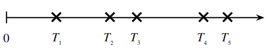
Count-Time Duality
Consider a Poisson process of emails arriving in an inbox at rate \(\lambda\) emails per hour. Let \(T_n\) be the time of arrival of the \(n\)th email (relative to some starting time \(0\)) and \(N_t\) be the number of emails that arrive in \([0,t]\).
Let’s find the distribution of \(T_1\). The event \(T_1 > t\), the event that you have to wait more than \(t\) hours to get the first email, is the same as the event \(N_t = 0\), which is the event that there are no emails in the first \(t\) hours. So,
[P(T_1 > t) = P(N_t = 0) = e^{-\lambda t}]
Therefore, \(P(T_1 \leq t) = 1 - e^{-\lambda t}\), and \(T_1\) follows an exponential distribution with parameter \(\lambda\).
By the memoryless property and similar reasoning, the interarrival times between emails are i.i.d. exponential random variables with parameter \(\lambda\), i.e., the differences \(T_n - T_{n-1}\) are i.i.d. exponential random variables with parameter \(\lambda\).
Order Statistics
Definition
Let’s say you have \(n\) i.i.d. random variables \(X_1, X_2, \dots, X_n\). If you arrange them from smallest to largest, the \(i\)th element in that list is the \(i\)th order statistic, denoted \(X_{(i)}\). So \(X_{(1)}\) is the smallest in the list and \(X_{(n)}\) is the largest in the list.
Note that the order statistics are dependent, e.g., learning \(X_{(4)} = 42\) gives us the information that \(X_{(1)},X_{(2)},X_{(3)}\) are \(\leq 42\) and \(X_{(5)},X_{(6)},\dots,X_{(n)}\) are \(\geq 42\).
Distribution
Taking \(n\) i.i.d. random variables \(X_1, X_2, \dots, X_n\) with CDF \(F(x)\) and PDF \(f(x)\), the CDF and PDF of \(X_{(i)}\) are: \(F_{X_{(i)}}(x) = P (X_{(i)} \leq x) = \sum_{k=i}^n {n \choose k} F(x)^k(1 - F(x))^{n - k}\) \(f_{X_{(i)}}(x) = n{n - 1 \choose i - 1}F(x)^{i-1}(1 - F(x))^{n-i}f(x)\)
Uniform Order Statistics
The \(j\)th order statistic of i.i.d. \(U_1,\dots,U_n \sim \text{Unif}(0,1)\) is \(U_{(j)} \sim \text{Beta}(j, n - j + 1)\).
Conditional Expectation
Conditioning on an Event
We can find \(E(Y|A)\), the expected value of \(Y\) given that event \(A\) occurred. A very important case is when \(A\) is the event \(X=x\). Note that \(E(Y|A)\) is a number.
For example:
- The expected value of a fair die roll, given that it is prime, is \(\frac{1}{3} \cdot 2 + \frac{1}{3} \cdot 3 + \frac{1}{3} \cdot 5 = \frac{10}{3}\).
- Let \(Y\) be the number of successes in \(10\) independent Bernoulli trials with probability \(p\) of success. Let \(A\) be the event that the first \(3\) trials are all successes. Then \(E(Y\|A) = 3 + 7p\) since the number of successes among the last \(7\) trials is \(\text{Bin}(7,p)\).
- Let \(T \sim \text{Expo}(1/10)\) be how long you have to wait until the shuttle comes. Given that you have already waited \(t\) minutes, the expected additional waiting time is \(10\) more minutes, by the memoryless property. That is, \(E(T\|T>t) = t + 10\).
Conditioning on a Random Variable
We can also find \(E(Y|X)\), the expected value of \(Y\) given the random variable \(X\). This is a function of the random variable \(X\). It is not a number except in certain special cases such as if \(X \perp Y\). To find \(E(Y|X)\), find \(E(Y|X = x)\) and then plug in \(X\) for \(x\).
For example:
- If \(E(Y\|X=x) = x^3+5x\), then \(E(Y\|X) = X^3 + 5X\).
- Let \(Y\) be the number of successes in \(10\) independent Bernoulli trials with probability \(p\) of success and \(X\) be the number of successes among the first \(3\) trials. Then \(E(Y\|X)=X+7p\).
- Let \(X \sim \mathcal{N}(0,1)\) and \(Y=X^2\). Then \(E(Y\|X=x) = x^2\) since if we know \(X=x\) then we know \(Y=x^2\). And \(E(X\|Y=y) = 0\) since if we know \(Y=y\) then we know \(X = \pm \sqrt{y}\), with equal probabilities (by symmetry). So \(E(Y\|X)=X^2\), \(E(X\|Y)=0\).
Properties of Conditional Expectation
- \(E(Y\|X) = E(Y)\) if \(X \perp Y\)
- \(E(h(X)W\|X) = h(X)E(W\|X)\) (taking out what’s known)
In particular, \(E(h(X)\|X) = h(X)\). - \(E(E(Y\|X)) = E(Y)\) (Adam’s Law, a.k.a. Law of Total Expectation)
Adam’s Law (a.k.a. Law of Total Expectation)
For any events \(A_1, A_2, \dots, A_n\) that partition the sample space: \(E(Y) = E(Y|A_1)P(A_1) + \dots + E(Y|A_n)P(A_n)\)
For the special case where the partition is \(A, A^c\), this says: \(E(Y) = E(Y|A)P(A) + E(Y|A^c)P(A^c)\)
Eve’s Law (a.k.a. Law of Total Variance)
\(\text{Var}(Y) = E(\text{Var}(Y|X)) + \text{Var}(E(Y|X))\)
MVN, LLN, CLT
Law of Large Numbers (LLN)
Let \(X_1, X_2, X_3, \dots\) be i.i.d. with mean \(\mu\). The sample mean is \(\bar{X}_n = \frac{X_1 + X_2 + X_3 + \dots + X_n}{n}\). The Law of Large Numbers states that as \(n \to \infty\), \(\bar{X}_n \to \mu\) with probability \(1\). For example, in flips of a coin with probability \(p\) of Heads, let \(X_j\) be the indicator of the \(j\)th flip being Heads. Then LLN says the proportion of Heads converges to \(p\) (with probability \(1\)).
Central Limit Theorem (CLT)
Approximation using CLT
We use \(\dot{\,\sim\,}\) to denote “is approximately distributed.” We can use the Central Limit Theorem to approximate the distribution of a random variable \(Y = X_1 + X_2 + \dots + X_n\) that is a sum of \(n\) i.i.d. random variables \(X_i\). Let \(E(Y) = \mu_Y\) and \(\text{Var}(Y) = \sigma^2_Y\). The CLT says: \(Y \dot{\,\sim\,} \mathcal{N}(\mu_Y, \sigma^2_Y)\)
If the \(X_i\) are i.i.d. with mean \(\mu_X\) and variance \(\sigma^2_X\), then \(\mu_Y = n \mu_X\) and \(\sigma^2_Y = n \sigma^2_X\). For the sample mean \(\bar{X}_n\), the CLT says: \(\bar{X}_n = \frac{1}{n}(X_1 + X_2 + \dots + X_n) \dot{\,\sim\,} \mathcal{N}(\mu_X, \frac{\sigma^2_X}{n})\)
Asymptotic Distributions using CLT
We use \(\xrightarrow{D}\) to denote “converges in distribution to” as \(n \to \infty\). The CLT says that if we standardize the sum \(X_1 + \dots + X_n\), then the distribution of the sum converges to \(\mathcal{N}(0,1)\) as \(n \to \infty\): \(\frac{1}{\sigma\sqrt{n}}(X_1 + \dots + X_n - n\mu_X) \xrightarrow{D} \mathcal{N}(0, 1)\) In other words, the CDF of the left-hand side goes to the standard Normal CDF, \(\Phi\). In terms of the sample mean, the CLT says: \(\frac{\sqrt{n}(\bar{X}_n - \mu_X)}{\sigma_X} \xrightarrow{D} \mathcal{N}(0, 1)\)
Markov Chains
Definition
A Markov chain is a random walk in a state space, which we will assume is finite, say \(\{1, 2, \dots, M\}\). We let \(X_t\) denote which element of the state space the walk is visiting at time \(t\). The Markov chain is the sequence of random variables tracking where the walk is at all points in time, \(X_0, X_1, X_2, \dots\). By definition, a Markov chain must satisfy the Markov property, which says that if you want to predict where the chain will be at a future time, if we know the present state then the entire past history is irrelevant. Given the present, the past and future are conditionally independent. In symbols: \(P(X_{n+1} = j | X_0 = i_0, X_1 = i_1, \dots, X_n = i) = P(X_{n+1} = j | X_n = i)\)
State Properties
A state is either recurrent or transient.
- If you start at a recurrent state, then you will always return back to that state at some point in the future. \textmusicalnote You can check-out any time you like, but you can never leave. \textmusicalnote
- Otherwise, you are at a transient state. There is some positive probability that once you leave, you will never return. \textmusicalnote You don’t have to go home, but you can’t stay here. \textmusicalnote
A state is either periodic or aperiodic.
- If you start at a periodic state of period \(k\), then the GCD of the possible numbers of steps it would take to return back is \(k > 1\).
- Otherwise, you are at an aperiodic state. The GCD of the possible numbers of steps it would take to return back is 1.
Transition Matrix
Let the state space be \(\{1,2,\dots,M\}\). The transition matrix \(Q\) is the \(M \times M\) matrix where element \(q_{ij}\) is the probability that the chain goes from state \(i\) to state \(j\) in one step:
| [q_{ij} = P(X_{n+1} = j | X_n = i)] |
To find the probability that the chain goes from state \(i\) to state \(j\) in exactly \(m\) steps, take the \((i, j)\) element of \(Q^m\):
| [q^{(m)}{ij} = P(X{n+m} = j | X_n = i)] |
If \(X_0\) is distributed according to the row vector PMF \(\vec{p}\), i.e., \(p_j = P(X_0 = j)\), then the PMF of \(X_n\) is \(\vec{p}Q^n\).
Chain Properties
A chain is irreducible if you can get from anywhere to anywhere. If a chain (on a finite state space) is irreducible, then all of its states are recurrent. A chain is periodic if any of its states are periodic, and is aperiodic if none of its states are periodic. In an irreducible chain, all states have the same period.
A chain is reversible with respect to \(\vec{s}\) if \(s_iq_{ij} = s_jq_{ji}\) for all \(i, j\). Examples of reversible chains include any chain with \(q_{ij} = q_{ji}\), with \(\vec{s} = (\frac{1}{M}, \frac{1}{M}, \dots, \frac{1}{M})\), and random walk on an undirected network.
Stationary Distribution
Let \(\vec{s} = (s_1, s_2, \dots, s_M)\) be a PMF (written as a row vector). We will call \(\vec{s}\) the stationary distribution for the chain if \(\vec{s}Q = \vec{s}\). As a consequence, if \(X_t\) has the stationary distribution, then all future \(X_{t+1}, X_{t + 2}, \dots\) also have the stationary distribution.
For irreducible, aperiodic chains, the stationary distribution exists, is unique, and \(s_i\) is the long-run probability of a chain being at state \(i\). The expected number of steps to return to \(i\) starting from \(i\) is \(1/s_i\).
To find the stationary distribution, you can solve the matrix equation \((Q' - I){\vec{s}\,}'= 0\). The stationary distribution is uniform if the columns of \(Q\) sum to 1.
Reversibility Condition Implies Stationarity: If you have a PMF \(\vec{s}\) and a Markov chain with transition matrix \(Q\), then \(s_iq_{ij} = s_jq_{ji}\) for all states \(i, j\) implies that \(\vec{s}\) is stationary.
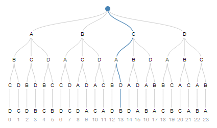
Random Walk on an Undirected Network
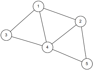
If you have a collection of nodes, pairs of which can be connected by undirected edges, and a Markov chain is run by going from the current node to a uniformly random node that is connected to it by an edge, then this is a random walk on an undirected network. The stationary distribution of this chain is proportional to the degree sequence (this is the sequence of degrees, where the degree of a node is how many edges are attached to it). For example, the stationary distribution of random walk on the network shown above is proportional to \((3,3,2,4,2)\), so it’s \((\frac{3}{14}, \frac{3}{14}, \frac{2}{14}, \frac{4}{14}, \frac{2}{14})\).
Continuous Distributions
Uniform Distribution
Let \(U\) be distributed \(\text{Unif}(a, b)\). We know the following:
- Properties of the Uniform: For a Uniform distribution, the probability of a draw from any interval within the support is proportional to the length of the interval.
-
Example: William throws darts really badly, so his darts are uniform over the whole room because they’re equally likely to appear anywhere. William’s darts have a Uniform distribution on the surface of the room. The Uniform is the only distribution where the probability of hitting in any specific region is proportional to the length/area/volume of that region, and where the density of occurrence in any one specific spot is constant throughout the whole support.
- PDF and CDF (top is Unif(0, 1), bottom is Unif(a, b))
For the Uniform distribution:
- Unif(0, 1):
- PDF: \(f(x) = \left\{ \begin{array}{lr} 1 & x \in [0, 1] \\ 0 & x \notin [0, 1] \end{array} \right.\)
- CDF: \(F(x) = \left\{ \begin{array}{lr} 0 & x < 0 \\ x & x \in [0, 1] \\ 1 & x > 1 \end{array} \right.\)
- Unif(a, b):
- PDF: \(f(x) = \left\{ \begin{array}{lr} \frac{1}{b-a} & x \in [a, b] \\ 0 & x \notin [a, b] \end{array} \right.\)
- CDF:
\(F(x) = \left\{
\begin{array}{lr}
0 & x < a \\
\frac{x-a}{b-a} & x \in [a, b] \\
1 & x > b
\end{array}
\right.\)
Normal Distribution
Let us say that X is distributed N(μ, σ^2). We know the following:
Central Limit Theorem The Normal distribution is ubiquitous because of the Central Limit Theorem, which states that the sample mean of i.i.d. r.v.s will approach a Normal distribution as the sample size grows, regardless of the initial distribution.
Location-Scale Transformation Every time we shift a Normal r.v. (by adding a constant) or rescale a Normal (by multiplying by a constant), we change it to another Normal r.v. For any Normal X ~ N(μ, σ^2), we can transform it to the standard N(0, 1) by the following transformation: Z = (X - μ) / σ ~ N(0, 1)
Standard Normal The Standard Normal, Z ~ N(0, 1), has mean 0 and variance 1. Its CDF is denoted by Φ.
Exponential Distribution
Let us say that X is distributed Expo(λ). We know the following:
Story You’re sitting on an open meadow right before the break of dawn, wishing that airplanes in the night sky were shooting stars, because you could really use a wish right now. You know that shooting stars come on average every 15 minutes, but a shooting star is not “due” to come just because you’ve waited so long. Your waiting time is memoryless; the additional time until the next shooting star comes does not depend on how long you’ve waited already.
Example The waiting time until the next shooting star is distributed Expo(4) hours. Here λ=4 is the rate parameter, since shooting stars arrive at a rate of 1 per 1/4 hour on average. The expected time until the next shooting star is 1/λ = 1/4 hour.
Expos as a rescaled Expo(1) Y ~ Expo(λ) ⇒ X = λY ~ Expo(1)
Memorylessness The Exponential Distribution is the only continuous memoryless distribution. The memoryless property says that for X ~ Expo(λ) and any positive numbers s and t: P(X > s + t | X > s) = P(X > t) Equivalently, (X - a | X > a) ~ Expo(λ)
Min of Expos If we have independent Xi ~ Expo(λi), then min(X1, …, Xk) ~ Expo(λ1 + λ2 + … + λk).
Max of Expos If we have i.i.d. Xi ~ Expo(λ), then max(X1, …, Xk) has the same distribution as Y1 + Y2 + … + Yk, where Yj ~ Expo(jλ) and the Yj are independent.
Gamma Distribution
Let us say that X is distributed Gam(a, λ). We know the following:
Story You sit waiting for shooting stars, where the waiting time for a star is distributed Expo(λ). You want to see n shooting stars before you go home. The total waiting time for the nth shooting star is Gam(n, λ).
Example You are at a bank, and there are 3 people ahead of you. The serving time for each person is Exponential with mean 2 minutes. Only one person at a time can be served. The distribution of your waiting time until it’s your turn to be served is Gam(3, 1/2).
Beta Distribution
Conjugate Prior of the Binomial In the Bayesian approach to statistics, parameters are viewed as random variables, to reflect our uncertainty. The prior for a parameter is its distribution before observing data. The posterior is the distribution for the parameter after observing data. Beta is the conjugate prior of the Binomial because if you have a Beta-distributed prior on p in a Binomial, then the posterior distribution on p given the Binomial data is also Beta-distributed. Consider the following two-level model: X | p ~ Bin(n, p) p ~ Beta(a, b) Then after observing X = x, we get the posterior distribution p | (X = x) ~ Beta(a + x, b + n - x)
Order statistics of the Uniform See Order Statistics.
Beta-Gamma relationship If X ~ Gam(a, λ), Y ~ Gam(b, λ), with X independent of Y, then:
- X / (X + Y) ~ Beta(a, b)
- X + Y independent of X / (X + Y)
Chi-Square Distribution
Let us say that X is distributed chi2_n. We know the following:
Story A Chi-Square(n) is the sum of the squares of n independent standard Normal r.v.s.
Properties and Representations
- \(X\) is distributed as \(Z1^2 + Z2^2 + ... + Zn^2\) for i.i.d. \(Z_i ~ N(0,1)\)\
- \[X ~ Gam(n/2, 1/2)\]
Discrete Distributions
Distributions for four sampling schemes
| Replace | No Replace | |
|---|---|---|
| Fixed # trials (\(n\)) | Binomial | Hypergeometric |
| (Bern if \(n = 1\)) | ||
| Draw until \(r\) success | Negative Binomial | Noncentral Hypergeometric |
| (Geometric if \(r = 1\)) |
Bernoulli Distribution
The Bernoulli distribution is the simplest case of the Binomial distribution, where we only have one trial (\(n=1\)). Let us say that X is distributed Bern(p). We know the following:
Story A trial is performed with probability p of “success”, and X is the indicator of success: 1 means success, 0 means failure.
Example Let X be the indicator of Heads for a fair coin toss. Then X follows the Bernoulli distribution with parameter p=1/2. Also, 1 - X follows the Bernoulli distribution with parameter p=1/2, representing the indicator of Tails.
Binomial Distribution
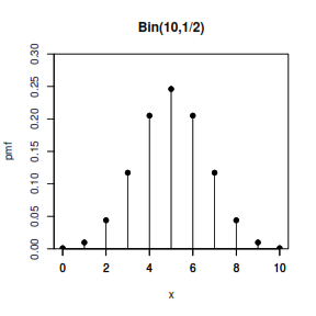
Let us say that X is distributed Bin(n, p). We know the following:
Story X is the number of “successes” that we will achieve in n independent trials, where each trial is either a success or a failure, each with the same probability p of success. X can be expressed as the sum of multiple independent Bernoulli random variables with parameter p. If X ~ Bin(n, p) and Xj ~ Bern(p), where all the Bernoullis are independent, then: X = X1 + X2 + X3 + … + Xn
Example If Jeremy Lin makes 10 free throws, and each throw independently has a 3/4 chance of getting in, then the number of successful throws is distributed as Bin(10, 3/4).
Properties
- Redefine success: If X ~ Bin(n, p), then n - X ~ Bin(n, 1 - p)
- Sum: If X ~ Bin(n, p) and Y ~ Bin(m, p) with X and Y being independent, then X + Y ~ Bin(n + m, p)
-
Conditional: If X ~ Bin(n, p) and Y ~ Bin(m, p) with X and Y being independent, then X (X + Y = r) ~ Hypergeometric(n, m, r) - Binomial-Poisson Relationship: Bin(n, p) is approximately Pois(np) if p is small.
- Binomial-Normal Relationship: Bin(n, p) is approximately N(np, np(1 - p)) if n is large and p is not near 0 or 1.
Geometric Distribution
Let us say that X is distributed Geom(p). We know the following:
Story X is the number of “failures” that we will achieve before we achieve our first success. The successes have a probability p.
Example If each Pokéball we throw has a 1/10 probability of catching Mew, then the number of failed Pokéballs before catching Mew follows the Geometric distribution with parameter p = 1/10.
The PMF of a Poisson distribution is given by:
[P(X = k) = \frac{e^{-\lambda}\lambda^k}{k!}]
where X is the random variable following a Poisson distribution, and λ is the average rate of events occurring per unit space or time.
Multivariate Distributions
Multinomial Distribution
Let us say that the vector \(\vec{X} = (X_1, X_2, X_3, \dots, X_k) \sim \text{Mult}_k(n, \vec{p})\) where \(\vec{p} = (p_1, p_2, \dots, p_k)\).
- Story: We have \(n\) items, which can fall into any one of the \(k\) buckets independently with the probabilities \(\vec{p} = (p_1, p_2, \dots, p_k)\).
- Example: Let us assume that every year, 100 students in the Harry Potter Universe are randomly and independently sorted into one of four houses with equal probability. The number of people in each of the houses is distributed \(\text{Mult}_4(100, \vec{p})\), where \(\vec{p} = (0.25, 0.25, 0.25, 0.25)\). Note that \(X_1 + X_2 + \dots + X_4 = 100\), and they are dependent.
- Joint PMF: For \(n = n_1 + n_2 + \dots + n_k\), the joint probability mass function is: \(P(\vec{X} = \vec{n}) = \frac{n!}{n_1!n_2!\dots n_k!}p_1^{n_1}p_2^{n_2}\dots p_k^{n_k}\)
- Marginal PMF, Lumping, and Conditionals: Marginally, \(X_i \sim \text{Bin}(n,p_i)\) since we can define “success” to mean category \(i\). If you lump together multiple categories in a Multinomial, then it is still Multinomial. Conditioning on some \(X_j\) also gives a Multinomial.
- Variances and Covariances: We have \(X_i \sim \text{Bin}(n, p_i)\) marginally, so \(\text{Var}(X_i) = np_i(1-p_i)\). Also, \(\text{Cov}(X_i, X_j) = -np_ip_j\) for $$i \neq j.
Multivariate Uniform Distribution
See the univariate Uniform for stories and examples. For the 2D Uniform on some region, probability is proportional to area. Every point in the support has equal density, of value \(1/\text{area of region}\). For the 3D Uniform, probability is proportional to volume.
Multivariate Normal (MVN) Distribution
A vector \(\vec{X} = (X_1, X_2, \dots, X_k)\) is Multivariate Normal if every linear combination is Normally distributed, i.e., \(t_1X_1 + t_2X_2 + \dots + t_kX_k\) is Normal for any constants \(t_1, t_2, \dots, t_k\). The parameters of the Multivariate Normal are the mean vector \(\vec{\mu} = (\mu_1, \mu_2, \dots, \mu_k)\) and the covariance matrix where the \((i, j)\) entry is \(\text{cov}(X_i, X_j)\).
- Properties: The Multivariate Normal has the following properties:
- Any subvector is also MVN.
- If any two elements within an MVN are uncorrelated, then they are independent.
- The joint PDF of a Bivariate Normal \((X,Y)\) with \(\mathcal{N}(0,1)\) marginal distributions and correlation \(\rho \in (-1,1)\) is: \(f_{X,Y}(x,y) = \frac{1}{2 \pi \tau} \exp\left(-\frac{1}{2 \tau^2} (x^2+y^2-2 \rho xy)\right),\) with \(\tau = \sqrt{1-\rho^2}\).
Distribution Properties
Important CDFs
- Standard Normal: \(\Phi\)
- Exponential(\(\lambda\)): \(F(x) = 1 - e^{-\lambda x}\), for \(x \in (0, \infty)\)
- Uniform(0,1): \(F(x) = x\), for \(x \in (0, 1)\)
Convolutions of Random Variables
A convolution of \(n\) random variables is simply their sum. For the following results, let \(X\) and \(Y\) be independent.
- \(X \sim \text{Pois}(\lambda_1)\), \(Y \sim \text{Pois}(\lambda_2)\) \(\longrightarrow X + Y \sim \text{Pois}(\lambda_1 + \lambda_2)\)
- \(X \sim \text{Bin}(n_1, p)\), \(Y \sim \text{Bin}(n_2, p)\) \(\longrightarrow X + Y \sim \text{Bin}(n_1 + n_2, p)\). \(\text{Bin}(n,p)\) can be thought of as a sum of i.i.d. \(\text{Bern}(p)\) random variables.
- \(X \sim \text{Gam}(a_1, \lambda)\), \(Y \sim \text{Gam}(a_2, \lambda)\) \(\longrightarrow X + Y \sim \text{Gam}(a_1 + a_2, \lambda)\). \(\text{Gam}(n,\lambda)\) with \(n\) an integer can be thought of as a sum of i.i.d. \(\text{Expo}(\lambda)\) random variables.
- \(X \sim \text{NBin}(r_1, p)\), \(Y \sim \text{NBin}(r_2, p)\) \(\longrightarrow X + Y \sim \text{NBin}(r_1 + r_2, p)\). \(\text{NBin}(r,p)\) can be thought of as a sum of i.i.d. \(\text{Geom}(p)\) random variables.
- \(X \sim \mathcal{N}(\mu_1, \sigma_1^2)\), \(Y \sim \mathcal{N}(\mu_2, \sigma_2^2)\) \(\longrightarrow X + Y \sim \mathcal{N}(\mu_1 + \mu_2, \sigma_1^2 + \sigma_2^2)\)
Special Cases of Distributions
- \(\text{Bin}(1, p) \sim \text{Bern}(p)\).
- \(\text{Beta}(1, 1) \sim \text{Unif}(0, 1)\).
- \(\text{Gam}(1, \lambda) \sim \text{Expo}(\lambda)\).
- \(\chi^2_n \sim \text{Gam}\left(\frac{n}{2}, \frac{1}{2}\right)\).
- \(\text{NBin}(1, p) \sim \text{Geom}(p)\).
[\textbf{Inequalities}]
-
Cauchy-Schwarz: \(|E(XY)| \leq \sqrt{E(X^2)E(Y^2)}\)
-
Markov: \(P(X \geq a) \leq \frac{E|X|}{a}\) for \(a>0\)
-
Chebyshev: \(P(|X - \mu| \geq a) \leq \frac{\sigma^2}{a^2}\) for \(E(X)=\mu\), \(\text{Var}(X) = \sigma^2\)
-
Jensen: \(E(g(X)) \geq g(E(X))\) for \(g\) convex; reverse if \(g\) is concave
[\textbf{Formulas}]
[\textbf{Geometric Series}]
[1 + r + r^2 + \dots + r^{n-1} = \sum_{k=0}^{n-1} r^k = \frac{1 - r^n}{1 -r}]
| [1 + r + r^2 + \dots = \frac{1}{1-r} \text{ if } | r | <1] |
[\textbf{Exponential Function ($e^x$)}]
[e^x = \sum_{n=0}^\infty \frac{x^n}{n!}= 1 + x + \frac{x^2}{2!} + \frac{x^3}{3!} + \dots = \lim_{n \rightarrow \infty} \left( 1 + \frac{x}{n} \right)^n]
[\textbf{Gamma and Beta Integrals}]
You can sometimes solve complicated-looking integrals by pattern-matching to a gamma or beta integral:
[\int_0^\infty x^{t-1}e^{-x}\, dx = \Gamma(t) \hspace{1 cm} \int_0^1 x^{a - 1}(1-x)^{b-1}\, dx = \frac{\Gamma(a)\Gamma(b)}{\Gamma(a + b)}]
Also, \(\Gamma(a+1) = a \Gamma(a)\), and \(\Gamma(n) = (n - 1)!\) if \(n\) is a positive integer.
[\textbf{Euler’s Approximation for Harmonic Sums}]
[1 + \frac{1}{2} + \frac{1}{3} + \dots + \frac{1}{n} \approx \log n + 0.577 \dots]
[\textbf{Stirling’s Approximation for Factorials}]
[n! \approx \sqrt{2\pi n}\left(\frac{n}{e}\right)^n]
Miscellaneous Definitions
Medians and Quantiles Let \(X\) have CDF \(F\). Then \(X\) has median \(m\) if \(F(m) \geq 0.5\) and \(P(X \geq m) \geq 0.5\). For \(X\) continuous, \(m\) satisfies \(F(m) = \frac{1}{2}\). In general, the \(a\)th quantile of \(X\) is \(\min \{x: F(x) \geq a\}\); the median is the case \(a = \frac{1}{2}\).
log Statisticians generally use \(\log\) to refer to natural log (i.e., base \(e\)).
i.i.d r.v.s Independent, identically-distributed random variables.
Example Problems
Calculating Probability
A textbook has \(n\) typos, which are randomly scattered amongst its \(n\) pages, independently. You pick a random page. What is the probability that it has no typos?
Solution
There is a \(\left(1 - \frac{1}{n}\right)\) probability that any specific typo isn’t on your page, and thus a \(\boxed{\left(1 - \frac{1}{n}\right)^n}\) probability that there are no typos on your page. For \(n\) large, this is approximately \(e^{-1} = \frac{1}{e}\).
Linearity and Indicators (1)
In a group of \(n\) people, what is the expected number of distinct birthdays (month and day)? What is the expected number of birthday matches?
Solution
Let \(X\) be the number of distinct birthdays and \(I_j\) be the indicator for the \(j\)th day being represented.
\(E(I_j) = 1 - P(\text{no one born on day }j) = 1 - \left(\frac{364}{365}\right)^n\)
By linearity, \(\boxed{E(X) = 365\left(1-\frac{364}{365}\right)^n}\).\ Now let \(Y\) be the number of birthday matches and \(J_i\) be the indicator that the \(i\)th pair of people have the same birthday. The probability that any two specific people share a birthday is \(\frac{1}{365}\), so \(\boxed{E(Y) = \frac{\binom{n}{2}}{365}}\).
Linearity and Indicators (2)
This problem is commonly known as the hat-matching problem. There are \(n\) people at a party, each with a hat. At the end of the party, they each leave with a random hat. What is the expected number of people who leave with the right hat?
Solution
Each hat has a \(\frac{1}{n}\) chance of going to the right person. By linearity, the average number of hats that go to their owners is \(\boxed{1}\).
Linearity and First Success
This problem is commonly known as the coupon collector problem. There are \(n\) coupon types. At each draw, you get a uniformly random coupon type. What is the expected number of coupons needed until you have a complete set?
Solution
Let \(N\) be the number of coupons needed; we want \(E(N)\). Let \(N = N_1 + \dots + N_n\), where \(N_1\) is the draws to get our first new coupon, \(N_2\) is the additional draws needed to draw our second new coupon, and so on. By the story of the First Success, \(N_2 \sim \text{FS}\left(\frac{n-1}{n}\right)\) (after collecting the first coupon type, there’s \(\frac{n-1}{n}\) chance you’ll get something new). Similarly, \(N_3 \sim \text{FS}\left(\frac{n-2}{n}\right)\), and \(N_j \sim \text{FS}\left(\frac{n-j+1}{n}\right)\). By linearity,
\(E(N) = E(N_1) + \dots + E(N_n) = \frac{n}{n} + \frac{n}{n-1} + \dots + \frac{n}{1} = \boxed{n\sum^n_{j=1} \frac{1}{j}}\) This is approximately \(n (\log(n) + 0.577)\) by Euler’s approximation.
Orderings of i.i.d. random variables
I call 2 UberX’s and 3 Lyfts at the same time. If the time it takes for the rides to reach me are i.i.d., what is the probability that all the Lyfts will arrive first?
Solution
Since the arrival times of the five cars are i.i.d., all \(5!\) orderings of the arrivals are equally likely. There are \(3!2!\) orderings that involve the Lyfts arriving first, so the probability that the Lyfts arrive first is \(\boxed{\frac{3!2!}{5!} = \frac{1}{10}}\). Alternatively, there are \(\binom{5}{3}\) ways to choose 3 of the 5 slots for the Lyfts to occupy, where each of the choices is equally likely. One of these choices has all 3 of the Lyfts arriving first, so the probability is \(\boxed{\frac{1}{5 \choose 3} = \frac{1}{10}}\).
Expectation of Negative Hypergeometric
What is the expected number of cards that you draw before you pick your first Ace in a shuffled deck (not counting the Ace)?
Solution
Consider a non-Ace. Denote this to be card \(j\). Let \(I_j\) be the indicator that card \(j\) will be drawn before the first Ace. Note that \(I_j=1\) says that \(j\) is before all 4 of the Aces in the deck. The probability that this occurs is \(\frac{1}{5}\) by symmetry. Let \(X\) be the number of cards drawn before the first Ace. Then \(X = I_1 + I_2 + \ldots + I_{48}\), where each indicator corresponds to one of the 48 non-Aces. Thus,
\(E(X) = E(I_1) + E(I_2) + \ldots + E(I_{48}) = \frac{48}{5} = \boxed{9.6}\).
Minimum and Maximum of RVs
What is the CDF of the maximum of \(n\) independent Unif(0,1) random variables?
Solution
Note that for r.v.s \(X_1,X_2,\dots,X_n\),
\(P(\min(X_1, X_2, \dots, X_n) \geq a) = P(X_1 \geq a, X_2 \geq a, \dots, X_n \geq a)\)
Similarly,
\(P(\max(X_1, X_2, \dots, X_n) \leq a) = P(X_1 \leq a, X_2 \leq a, \dots, X_n \leq a)\)
We will use this principle to find the CDF of \(U_{(n)}\), where \(U_{(n)} = \max(U_1, U_2, \dots, U_n)\) and \(U_i \sim \text{Unif}(0, 1)\) are i.i.d. \(\ P(\max(U_1, U_2, \dots, U_n) \leq a) = P(U_1 \leq a, U_2 \leq a, \dots, U_n \leq a) = P(U_1 \leq a)P(U_2 \leq a)\dots P(U_n \leq a) = \boxed{a^n}\)
for \(0<a<1\) (and the CDF is \(0\) for \(a \leq 0\) and \(1\) for \(a \geq 1\)).
Pattern-matching with \(e^x\) Taylor series
Solution
For \(X \sim \text{Pois}(\lambda)\), find \(E\left(\frac{1}{X+1}\right)\). By LOTUS,
\(E\left(\frac{1}{X+1}\right) = \sum_{k=0}^\infty \frac{1}{k+1} \frac{e^{-\lambda}\lambda^k}{k!} = \frac{e^{-\lambda}}{\lambda}\sum_{k=0}^\infty \frac{\lambda^{k+1}}{(k+1)!} = \boxed{\frac{e^{-\lambda}}{\lambda}(e^\lambda-1)}\)
Adam’s Law and Eve’s Law
William really likes speedsolving Rubik’s Cubes. But he’s pretty bad at it, so sometimes he fails. On any given day, William will attempt \(N \sim \text{Geom}(s)\) Rubik’s Cubes. Suppose each time, he has probability \(p\) of solving the cube, independently. Let \(T\) be the number of Rubik’s Cubes he solves during a day. Find the mean and variance of \(T\).
Solution
Note that \(T|N \sim \text{Bin}(N,p)\). So by Adam’s Law,
\(E(T) = E(E(T|N)) = E(Np) = \boxed{\frac{p (1-s)}{s}}\)
Similarly, by Eve’s Law, we have
\(\text{Var}(T) = E(\text{Var}(T|N)) + \text{Var}(E(T|N)) = E(Np(1-p)) + \text{Var}(Np) = \frac{p(1-p)(1-s)}{s} + \frac{p^2(1-s)}{s^2} = \boxed{\frac{p(1-s)(p+s(1-p))}{s^2}}\)
MGF – Distribution Matching
(Continuing the Rubik’s Cube question above) Find the MGF of \(T\). What is the name of this distribution and its parameter(s)?
Solution
By Adam’s Law, we have
\(E(e^{tT}) = E(E(e^{tT}|N)) = E((pe^t + q)^N) = s\sum_{n=0}^\infty(pe^t + 1-p)^n(1-s)^n =\frac{s}{1-(1-s)(pe^t+1-p)} =\frac{s}{s+(1-s)p-(1-s)pe^t}\)
Intuitively, we would expect that \(T\) is distributed Geometrically since \(T\) is just a filtered version of \(N\), which itself is Geometrically distributed. The MGF of \(X\sim\text{Geom}(\theta)\) is \(E(e^{tX}) = \frac{\theta}{1-(1-\theta) e^t}\)
So, we would want to try to get our MGF into this form to identify what \(\theta\) is. Taking our original MGF, it would appear that dividing by \(s+(1-s)p\) would allow us to do this. Therefore, we have that
\(E(e^{tT}) = \frac{s}{s+(1-s)p - (1-s)pe^t} = \frac{\frac{s}{s+(1-s)p}}{1-\frac{(1-s)p}{s+(1-s)p}e^t}\)
By pattern-matching, it thus follows that \(\boxed{T \sim \text{Geom}(\theta)}\) where
\(\boxed{\theta = \frac{s}{s+(1-s)p}}\)
MGF – Finding Moments
Find \(E(X^3)\) for \(X \sim \text{Expo}(\lambda)\) using the MGF of \(X\).
Solution
The MGF of an \(\text{Expo}(\lambda)\) is \(M(t) = \frac{\lambda}{\lambda-t}\). To get the third moment, we can take the third derivative of the MGF and evaluate at \(t=0\):
\(\boxed{E(X^3) = \frac{6}{\lambda^3}}\)
But a much nicer way to use the MGF here is via pattern recognition: note that \(M(t)\) looks like it came from a geometric series:
\(\frac{1}{1-\frac{t}{\lambda}} = \sum^{\infty}_{n=0} \left(\frac{t}{\lambda}\right)^n = \sum^{\infty}_{n=0} \frac{n!}{\lambda^n} \frac{t^n}{n!}\)
The coefficient of \(\frac{t^n}{n!}\) here is the \(n\)th moment of \(X\), so we have \(E(X^n) = \frac{n!}{\lambda^n}\) for all nonnegative integers \(n\).
Markov chains (1)
Suppose \(X_n\) is a two-state Markov chain with transition matrix\ \(Q = \begin{bmatrix} 1-\alpha & \alpha \\ \beta & 1-\beta \end{bmatrix}\)
Find the stationary distribution \(\vec{s} = (s_0, s_1)\) of \(X_n\) by solving \(\vec{s} Q = \vec{s}\), and show that the chain is reversible with respect to \(\vec{s}\).\Solution
The equation \(\vec{s}Q = \vec{s}\) says that
\(s_0 = s_0(1-\alpha) + s_1 \beta \text{ and } s_1 = s_0(\alpha) + s_0(1-\beta)\)
By solving this system of linear equations, we have
\(\boxed{\vec{s} = \left(\frac{\beta}{\alpha+\beta}, \frac{\alpha}{\alpha+\beta}\right)}\)
To show that the chain is reversible with respect to \(\vec{s}\), we must show \(s_i q_{ij} = s_j q_{ji}\) for all \(i, j\). This is done if we can show \(s_0 q_{01} = s_1 q_{10}\). And indeed,
\(s_0 q_{01} = \frac{\alpha\beta}{\alpha+\beta} = s_1 q_{10}\)
Markov chains (2)
William and Sebastian play a modified game of Settlers of Catan, where every turn they randomly move the robber (which starts on the center tile) to one of the adjacent hexagons.
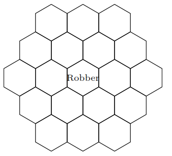
1. Is this Markov chain irreducible? Is it aperiodic?
Solution
Yes to both. The Markov chain is irreducible because it can get from anywhere to anywhere else. The Markov chain is aperiodic because the robber can return back to a square in 2, 3, 4, 5, … moves, and the greatest common divisor (GCD) of those numbers is 1.
2. What is the stationary distribution of this Markov chain?
Solution
Since this is a random walk on an undirected graph, the stationary distribution is proportional to the degree sequence. The degree for the corner pieces is 3, the degree for the edge pieces is 4, and the degree for the center pieces is 6. To normalize this degree sequence, we divide by its sum. The sum of the degrees is 6(3) + 6(4) + 7(6) = 84. Thus, the stationary probability of being on a corner is 3/84 = 1/28, on an edge is 4/84 = 1/21, and in the center is 6/84 = 1/14.
3. What fraction of the time will the robber be in the center tile in this game, in the long run?
Solution
By the above, 1/14.
4. What is the expected amount of moves it will take for the robber to return to the center tile?
Solution
Since this chain is irreducible and aperiodic, to get the expected time to return we can just invert the stationary probability. Thus, on average it will take 14 turns for the robber to return to the center tile.
Problem-Solving Strategies
Contributions from Jessy Hwang, Yuan Jiang, Yuqi Hou
-
Getting started. Start by defining relevant events and random variables. (“Let \(A\) be the event that I pick the fair coin”; “Let \(X\) be the number of successes.”) Clear notion is important for clear thinking! Then decide what it is that you’re supposed to be finding, in terms of your notation (“I want to find \(P(X=3|A)\)”). Think about what type of object your answer should be (a number? A random variable? A PMF? A PDF?) and what it should be in terms of.
Try simple and extreme cases. To make an abstract experiment more concrete, try drawing a picture or making up numbers that could have happened. Pattern recognition: does the structure of the problem resemble something we’ve seen before? -
Calculating probability of an event. Use counting principles if the naive definition of probability applies. Is the probability of the complement easier to find? Look for symmetries. Look for something to condition on, then apply Bayes’ Rule or the Law of Total Probability.
-
Finding the distribution of a random variable. First make sure you need the full distribution not just the mean (see next item). Check the support of the random variable: what values can it take on? Use this to rule out distributions that don’t fit. Is there a story for one of the named distributions that fits the problem at hand? Can you write the random variable as a function of an r.v. with a known distribution, say \(Y = g(X)\)?
-
Calculating expectation. If it has a named distribution, check out the table of distributions. If it’s a function of an r.v. with a named distribution, try LOTUS. If it’s a count of something, try breaking it up into indicator r.v.s. If you can condition on something natural, consider using Adam’s law.
-
Calculating variance. Consider independence, named distributions, and LOTUS. If it’s a count of something, break it up into a sum of indicator r.v.s. If it’s a sum, use properties of covariance. If you can condition on something natural, consider using Eve’s Law.
-
Calculating \(E(X^2)\). Do you already know \(E(X)\) or \(\text{Var}(X)\)? Recall that \(\text{Var}(X) = E(X^2) - (E(X))^2\). Otherwise try LOTUS.
-
Calculating covariance. Use the properties of covariance. If you’re trying to find the covariance between two components of a Multinomial distribution, \(X_i, X_j\), then the covariance is \(-np_ip_j\) for \(i \neq j\).
-
Symmetry. If \(X_1,\dots,X_n\) are i.i.d., consider using symmetry.
-
Calculating probabilities of orderings. Remember that all \(n!\) ordering of i.i.d. continuous random variables \(X_1,\dots,X_n\) are equally likely.
-
Determining independence. There are several equivalent definitions. Think about simple and extreme cases to see if you can find a counterexample.
-
Do a painful integral. If your integral looks painful, see if you can write your integral in terms of a known PDF (like Gamma or Beta), and use the fact that PDFs integrate to \(1\)?
-
Before moving on. Check some simple and extreme cases, check whether the answer seems plausible, check for biohazards.
Biohazards
Contributions from Jessy Hwang
-
Don’t misuse the naive definition of probability. When answering “What is the probability that in a group of 3 people, no two have the same birth month?”, it is not correct to treat the people as indistinguishable balls being placed into 12 boxes, since that assumes the list of birth months {January, January, January} is just as likely as the list {January, April, June}, even though the latter is six times more likely.
-
Don’t confuse unconditional, conditional, and joint probabilities. In applying \(P(A|B) = \frac{P(B|A)P(A)}{P(B)}\), it is not correct to say “\(P(B) = 1\) because we know \(B\) happened”; \(P(B)\) is the prior probability of \(B\). Don’t confuse \(P(A|B)\) with \(P(A,B)\).
-
Don’t assume independence without justification. In the matching problem, the probability that card 1 is a match and card 2 is a match is not \(1/n^2\). Binomial and Hypergeometric are often confused; the trials are independent in the Binomial story and dependent in the Hypergeometric story.
-
Don’t forget to do sanity checks. Probabilities must be between \(0\) and \(1\). Variances must be \(\geq 0\). Supports must make sense. PMFs must sum to \(1\). PDFs must integrate to \(1\).
-
Don’t confuse random variables, numbers, and events. Let \(X\) be an r.v. Then \(g(X)\) is an r.v. for any function \(g\). In particular, \(X^2\), \(|X|\), \(F(X)\), and \(I_{X>3}\) are r.v.s. \(P(X^2 < X | X \geq 0)\), \(E(X)\), \(\text{Var}(X)\), and \(g(E(X))\) are numbers. \(X = 2\) and \(F(X) \geq -1\) are events. It does not make sense to write \(\int_{-\infty}^\infty F(X) dx\), because \(F(X)\) is a random variable. It does not make sense to write \(P(X)\), because \(X\) is not an event.
-
Don’t confuse a random variable with its distribution. To get the PDF of \(X^2\), you can’t just square the PDF of \(X\). The right way is to use transformations. To get the PDF of \(X + Y\), you can’t just add the PDF of \(X\) and the PDF of \(Y\). The right way is to compute the convolution.
-
Don’t pull non-linear functions out of expectations. \(E(g(X))\) does not equal \(g(E(X))\) in general. The St. Petersburg paradox is an extreme example. See also Jensen’s inequality. The right way to find \(E(g(X))\) is with LOTUS.
Distributions in R
| Command | What it does |
|---|---|
help(distributions) |
shows documentation on distributions |
dbinom(k,n,p) |
PMF \(P(X=k)\) for \(X \sim \text{Bin}(n,p)\) |
pbinom(x,n,p) |
CDF \(P(X \leq x)\) for \(X \sim \text{Bin}(n,p)\) |
qbinom(a,n,p) |
\(a\)th quantile for \(X \sim \text{Bin}(n,p)\) |
rbinom(r,n,p) |
vector of \(r\) i.i.d. \(\text{Bin}(n,p)\) r.v.s |
dgeom(k,p) |
PMF \(P(X=k)\) for \(X \sim \text{Geom}(p)\) |
dhyper(k,w,b,n) |
PMF \(P(X=k)\) for \(X \sim \text{HGeom}(w,b,n)\) |
dnbinom(k,r,p) |
PMF \(P(X=k)\) for \(X \sim \text{NBin}(r,p)\) |
dpois(k,r) |
PMF \(P(X=k)\) for \(X \sim \text{Pois}(r)\) |
dbeta(x,a,b) |
PDF \(f(x)\) for \(X \sim \text{Beta}(a,b)\) |
dchisq(x,n) |
PDF \(f(x)\) for \(X \sim \chi^2_n\) |
dexp(x,b) |
PDF \(f(x)\) for \(X \sim \text{Expo}(b)\) |
dgamma(x,a,r) |
PDF \(f(x)\) for \(X \sim \text{Gam}(a,r)\) |
dlnorm(x,m,s) |
PDF \(f(x)\) for \(X \sim \mathcal{LN}(m,s^2)\) |
dnorm(x,m,s) |
PDF \(f(x)\) for \(X \sim \mathcal{N}(m,s^2)\) |
dt(x,n) |
PDF \(f(x)\) for \(X \sim t_n\) |
dunif(x,a,b) |
PDF \(f(x)\) for \(X \sim \text{Unif}(a,b)\) |
The table above gives R commands for working with various named distributions. Commands analogous to pbinom, qbinom, and rbinom work for the other distributions in the table. For example, pnorm, qnorm, and rnorm can be used to get the CDF, quantiles, and random generation for the Normal. For the Multinomial, dmultinom can be used for calculating the joint PMF and rmultinom can be used for generating random vectors. For the Multivariate Normal, after installing and loading the mvtnorm package, dmvnorm can be used for calculating the joint PDF and rmvnorm can be used for generating random vectors.
Recommended Resources
- Introduction to Probability Book
- Stat 110 Online
- Stat 110 Quora Blog
- Quora Probability FAQ
- R Studio
- LaTeX File: github.com/wzchen/probability_cheatsheet
Please share this cheatsheet with friends! wzchen.com/probability-cheatsheet
Table of Distributions
| Distribution | PMF/PDF and Support | Expected Value | Variance | MGF |
|---|---|---|---|---|
| Bernoulli | \(P(X=1) = p\) \(P(X=0) = q=1-p\) |
\(p\) | \(pq\) | \(q + pe^t\) |
| Binomial | \(P(X=k) = {n \choose k}p^k q^{n-k}\) | \(np\) | \(npq\) | \((q + pe^t)^n\) |
| Geometric | \(P(X=k) = q^kp\) | \(q/p\) | \(q/p^2\) | \(\frac{p}{1-qe^t}, \, qe^t < 1\) |
| Negative Binomial | \(P(X=n) = {r + n - 1 \choose r -1}p^rq^n\) | \(rq/p\) | \(rq/p^2\) | \((\frac{p}{1-qe^t})^r, \, qe^t < 1\) |
| Hypergeometric | \(P(X=k) = \frac{w \choose k}{b \choose n-k}{w + b \choose n}\) | \(\mu = \frac{nw}{b+w}\) | \(\left(\frac{w+b-n}{w+b-1} \right) n\frac{\mu}{n}(1 - \frac{\mu}{n})\) | messy |
| Poisson | \(P(X=k) = \frac{e^{-\lambda}\lambda^k}{k!}\) | \(\lambda\) | \(\lambda\) | \(e^{\lambda(e^t-1)}\) |
| Uniform | \(f(x) = \frac{1}{b-a}\) | \(\frac{a+b}{2}\) | \(\frac{(b-a)^2}{12}\) | \(\frac{e^{tb}-e^{ta}}{t(b-a)}\) |
| Normal | \(f(x) = \frac{1}{\sigma \sqrt{2\pi}} e^{-\frac{(x - \mu)^2}{(2 \sigma^2)}}\) | \(\mu\) | \(\sigma^2\) | \(e^{t\mu + \frac{\sigma^2t^2}{2}}\) |
| Exponential | \(f(x) = \lambda e^{-\lambda x}\) | \(\frac{1}{\lambda}\) | \(\frac{1}{\lambda^2}\) | \(\frac{\lambda}{\lambda - t}, \, t < \lambda\) |
| Gamma | \(f(x) = \frac{1}{\Gamma(a)}(\lambda x)^ae^{-\lambda x}\frac{1}{x}\) | \(\frac{a}{\lambda}\) | \(\frac{a}{\lambda^2}\) | \(\left(\frac{\lambda}{\lambda - t}\right)^a, \, t < \lambda\) |
| Beta | \(f(x) = \frac{\Gamma(a+b)}{\Gamma(a)\Gamma(b)}x^{a-1}(1-x)^{b-1}\) | \(\mu = \frac{a}{a + b}\) | \(\frac{\mu(1-\mu)}{(a + b + 1)}\) | messy |
| Log-Normal | \(\frac{1}{x\sigma \sqrt{2\pi}}e^{-(\log x - \mu)^2/(2\sigma^2)}\) | \(\theta = e^{ \mu + \sigma^2/2}\) | \(\theta^2 (e^{\sigma^2} - 1)\) | doesn’t exist |
| Chi-Square | \(\frac{1}{2^{n/2}\Gamma(n/2)}x^{n/2 - 1}e^{-x/2}\) | \(n\) | \(2n\) | \((1 - 2t)^{-n/2}, \, t < 1/2\) |
| Student-\(t\) | \(\frac{\Gamma((n+1)/2)}{\sqrt{n\pi} \Gamma(n/2)} (1+x^2/n)^{-(n+1)/2}\) | \(0\) if \(n>1\) | \(\frac{n}{n-2}\) if \(n>2\) | doesn’t exist |
Key Points
Permutations and Combinations
Overview
Teaching: min
Exercises: minQuestions
what are permutations and combinations
Objectives
Apply Fundamental Counting Principle
Apply Permutations
Apply Combinations
Concepts / Definitions
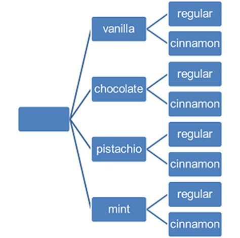
The Fundamental Counting Principle states that if one event has \(m\) possible outcomes and a second independent event has \(n\) possible outcomes, then there are \(m\) x \(n\) total possible outcomes for the two events together.
If you have four flavors of ice cream and two types of cones, then ther are \(4 * 2 = 8\) possible combinations.
In mathematics, the factorial of a non-negative integer \(n\), denoted by \(n!\), is the product of all positive integers less than or equal to \(n\). \(n! = n(n-1)(n-2)(n-3)\ ...\ (2)(1)\) By definition, \(0! = 1\).
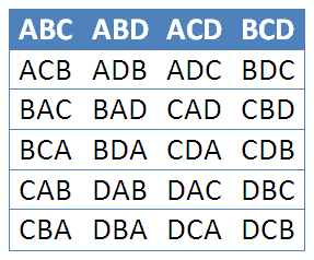
Permutations are the number of ways a set of \(n\) distinguishable objects can be arranged in order.
\(4!\) = 24 ways to order four items
The number of permutations on \(n\) objects taken \(r\) at a time is given by \(P\binom{n}{r} = P(n, r) = nPr = \frac{n!}{(n-r)!}\)
The number of ways \(n\) items can be ordered with replacement \(r\) times is \(n^r\)
\(\frac{4!}{(4-3)!}\) = 24 ways of selecting and ordering 3 or 4 letters, but only 4 ways if order does not matter.
Combinations are the number of ways selecting \(r\) items from a group of \(n\) items where order does not matter.
To take out all the ways \(r\) can happen, we divide out all the ways \(r!\) can happen.
The number of combinitions of \(n\) objects taken \(r\) at a time is given by
\(C\binom{n}{r} = C(n, r) = nCr = \frac{n!}{r!(n-r)!}\)
\(\implies\) Also called \(n\) choose \(k\), noted \(\binom{n}{k} = \frac{n!}{k!(n-k)!}\)
Counting Subsets of an \(n\)-Set
Consider a binomial situation, where there is a yes or no, success or failure, possibility happening \(n\) times. The number of ways this can happen is \(2^n\). There are \(2^n\) subsets of a set with \(n\) objects.
Exercises
1. A four-volume work is placed in random order on a bookshelf. What is the probability of the volumes being in proper order from left to right or from right to left?
Solution
If you have four volumes, and the question is what order to place them in, the question is a simple permutation problem. There are 4 possibilities for the first, 3 for the second, 2 for the third and only one for the last, making the number of permutations of the books 24. Only one order has them in ascending order and only one order will have them in descending order. Thus: \(P=\frac{2}{24}=\frac{1}{12}\label{answer1.1}\)
2.A wooden cube with painted faces is sawed up into 1000 little cubes, all of the same size. The little cubes are then mixed up, and one is chosen at random. What is the probability of its having just 2 painted faces?
Solution
The wooden cube is made of \(10^3\) cubes implying a 10x10x10 cube. The cubes that have two faces painted will be the edges which are not on a corner. Thus, since there are 12 edges of 10 cubes each, 8 of which are not corners, that implies we have 96 edges. 96 thus becomes our number of desireable outcomes and 1000 has always been the total number of outcomes: \(P=\frac{96}{1000} = 0.096\label{answer1.2}\)
3. A batch of n manufactured items contains k defective items. Suppose m items are selected at random from the batch. What is the probability that l of these items are defective?
Solution
If there are \(n\) total items and \(k\) of them are defective. We select \(m\) and want to know the probability of \(l\) of them being defective ones. There are \(\binom{n}{m}\) possible ways to chose \(m\) different items from the population of \(n\) items which will be our denominator. Now we need to know how many of those possibilities have \(l\) bad ones in them for our numerator. If there’s \(k\) total defective ones, then there are \(\binom{k}{l}\) \(P = \frac{\binom{k}{l}}{\binom{n}{m}}\label{answer1.3}\)
4. Ten books are placed in random order on a bookshelf. Find the probability of three given books being side by side.
Solution
There are \(10!\) possible ways to order the ten books. You can imagine that since the three books have to take up three adjacent positions, there are 8 possible locations for the three books to be ordered. Taking just the first position (that being the first three “Slots”), there are 6 ways to order the desired books and then \(7!\) ways to order the remaining books. Thus there are \(8 \cdot{} 6 \cdot{} 7!\) desirable orders giving us a probability of \(P=\frac{8 \cdot{} 6 \cdot{} 7!}{10!}=\frac{1}{15}\label{answer1.4}\)
5. One marksman has an 80% probability of hitting a target, while another has only a 70% probability of hitting the target. What is the probability of the target being hit (at least once) if both marksman fire at it simultaneously?
Solution
There are 4 possibilities to consider here: neither hits, one or the other hits and both hits. While it may be tempting to calculate the probability of each event, since we only care about the probability of at least one hitting the target, we need only calculate the probability that no one hits and subtract that from 1. The first marksman has an \(.8\) probability of hitting meaning he has a missing probability of .2; similarly the second marksman has a .7 chance of hitting and a .3 chance of missing. Thus, the probability of both one and two missing is the product of the two missing probabilities: \(.2*.3=.06\) \(P=1-.06=.94\label{answer1.5}\)
6. Suppose n people sit down at random and independently of each other in an auditorium containing n + k seats. What is the probability that m seats specified in advance (m < n) will be occupied?
Solution
The total number of ways \(n+k\) seats can be occupied by \(n\) people is \(\binom{n+k}{n}=\frac{(n+k)!}{n!k!}\) but once again the difficult part is finding the total number of desirable outcomes. If you were to specify \(m\) seats, you effectively divide the auditorium into two buckets so we need to find the number of ways to partition people into those two buckets which will give us the numerator, \(\binom{n+k}{m}=\frac{(n+k)!}{m!(n+k-m)!}\)
\(P=\frac{(n+k)!}{m!(n+k-m)!}\frac{n!k!}{(n+k)!}\)
\(=\frac{n!k!}{m!(n+k-m)!}\)
7. Three cards are drawn at random from a full deck. What is the probability of getting a three, a seven and an ace?
Solution
Again, the number of ways to get three cards from a 52 card deck is \(\binom{52}{3}\). Since there are 4 each of sevens, threes and aces, there are $4^3$ desirable hands. \(P=\frac{4^3}{\frac{52!}{3!49!}}=\frac{16}{5525}=0.00289593 \label{answer1.7}\) Which it is worth pointing out, is no different than any other 3-card hand of three different cards.
8. What is the probability of being able to form a triangle from three segments chosen at random from five line segments of lengths 1, 3, 5, 7 and 9?
Hint. A triangle cannot be formed if one segment is longer than the sum of the other two.
Solution
If you indiscriminately chose 3 line segments from our bank of 5, you have \(\binom{5}{3}=10\) total possibilities for triangles.
When you look at the bank \((1, 3, 5, 7, 9)\), however, you have to make sure that no two segments are longer than the third segment, otherwise making a triangle is impossible.
The brute-force way to do this is start with 1 and realize there’s no triangle that can be formed with 1.
Then, looking at 3, you realize that you can do \((3, 5, 7)\) and \((3, 7, 9).\ Starting now with 5, you can do only\)(5, 7, 9)\(\ At this point, you realize you're done and that the answer is plain to see\)P=\frac{3}{10}=.3\label{answer1.8}$$
9. Suppose a number from 1 to 1000 is selected at random. What is the probability that the last two digits of its cube are both 1?
Hint There is no need to look through a table of cubes.
Solution
We could do this problem in 5 minutes of programming and an instant of computation but that’s not the point! We need to think our way through this one. How many cubes of the numbers between 1 and 1000, have 11 for the last two digits. Luckily, each cube is unique so there’s no complications there: only 1000 possibilities. Let’s break down the number we’re cubing into two parts, one that encapsulates the part less than 100 and then the rest of the number \(n=a+b=100c+b\) Now, just for fun, let’s cube than number \(n^3=(100c+b)^3=b^3+300 b^2 c+30000 b c^2+1000000 c^3\) Clearly the only term here that will matter to the last two digits of the cube is \(b\), the part less than 100. Now we can reduce our now size 100 subspace by a great deal if you realize that in order for a number’s cube to end in 1, the last number in the cube will need to be 1, leaving us: (1, 11, 21, 31, 41, 51, 61, 71, 81, 91). At this point I recommend just cubing all the numbers and realizing that only \(71^3=357911\) fulfills the requirements giving only one desirable outcome per century(71, 171, 271 etc.) \(P=\frac{10}{1000}=.01\label{answer1.9}\)
10. Find the probability that a randomly selected positive integer will give a number ending in 1 if it is
a) Squared ; b) Raised to the fourth power; c) Multiplied by an arbitrary positive integer. Hint. It is enough to consider one-digit numbers.
Solution
Now we want to know about all positive integers but just the last digit and the probability that the last digit is one. To prove that we can use the hint given, we’ll split the integer into the past less than 10 and the part greater than 10. \(n=10a+b\)
a–Squared
\(n^2=100a^2+10ab+b^2\) OK, so clearly only \(b^2\) contributes to the last digit. At this point... just do the squaring especially since it’s something you can do in your head. (1, 2, 3, 4, 5, 6, 7, 8, 9)\(\rightarrow\)(1, 4, 9, 16, 25, 36, 49, 64, 81) therefore there are two desireable outcomes for every decade of random positive integers.
\(P=\frac{2}{10}=.2\)b–fourth-powered
\(n^4=100000000 a^4+4000000 a^3 b+60000 a^2 b^2+400 a b^3+b^4\) Great, once again, just \(b^4\). Now, doing the forth power is a little harder so let’s reason through and reduce the subspace. Clearly, only odd numbers will contribute since any power of an even number is again an even number. Now, let’s just do the arithmetic. (1, 3, 5, 7, 9)\(\rightarrow\)(1, 81, 625, 2401, 6561) giving us 4 desirable outcomes per decade of random numbers
\(P=\frac{4}{10}=.4\)c–multiplied by random positive number
\(n*r=(10a+b)r\) Now let’s let $r$ be a similar integer as n \(n*r=(10a+b)(10c+d)=100ac+10(bc+ad)+bd\) So we just need to consider the first two digits of both the random number and the arbitrary number. This leaves us with $10^2$ possibilities; \(5^2\) possible desirable outcomes once we exclude even numbers: (1, 3, 5, 7, 9). Once again we resort to brute force by just defining the above as a vector and multiplying the transpose of that vector by the vector. The only desirable outcomes turn out to be (1*1, 9*9, 7*3, 3*7), giving four desirable outcomes per century.
\(P=\frac{4}{100}=.04\)
11. One of the numbers 2, 4, 6, 7, 8, 11, 12 and 13 is chosen at random as the numerator of a fraction, and then one of the remaining numbers is chosen at random as the denominator of the fraction. What is the probability of the fraction being in lowest terms?
Solution
Here we are given 8 possible numbers (2, 4, 6, 7, 8, 11, 12, 13) and are told that it making a random fraction out of two of the numbers. There are \(\binom{8}{2}=28\) possible pairs but since \(\frac{a}{b} \neq \frac{b}{a}\), we multiply that by two to get the total number of fractions we can get from these numbers as being 56. Looking at the numbers given, 7, 11 and 13 are all prime and all the others are divisible by two; therefore only the fractions that contain one or more prime numbers will be in lowest terms. The number 7 can be in 7 different pairs with the other numbers which makes for 14 fractions. 11 can be in 6 pairs or 12 fractions (since we already counted 7) and similarly, 13 can be in 10 uncounted fractions giving 36 possible fractions in lowest terms.
\(P=\frac{36}{56}=\frac{9}{14}\label{answer1.11}\)
12. The word “drawer” is spelled with six scrabble tiles. The tiles are then randomly rearranged. What is the probability of the rearranged tiles spelling the word “reward?»
Solution
The word drawer has 6 letters and there are \(6!=720\) possible ways of arranging the letters. It is then natural to say there’s only one way to spell reward correctly and thus the probability of spelling it correctly after a random reordering is \(1/720\) BUT there is a complication in that the two of our letters are the same, meaning there are to distinct arrangement of our distinguishable tiles that will give us the proper spelling. \(P=\frac{2}{720} = \frac{1}{360}\label{answer1.12}\)
13. In throwing 6n dice, what is the probability of getting each face n times? Use Stirling’s formula to estimate this probability for large n.
Solution
For any die, there are 6 different possibilities. Since one dice’s outcome does not depend on another’s, that means that for a roll of \(6n\) die, there are \(6^{6n}\) different possible outcomes for the dice rolls. Now for desirable outcomes, we want each of the 6 faces to show up n times. To accomplish this, we just count the number of ways to apportion \(6n\) things into 6 groups of $n$ each or \(\frac{(6n)!}{(n!)^6}\) which, given Stirling’s approximation \(n! \approx \sqrt{2 \pi n} n^n e^{-n}\) gives us for large \(n\) \(\frac{(6n)!}{(n!)^6} \approx \sqrt{2 \pi 6n} (6n)^{6n} e^{-6n} * \frac{1}{(\sqrt{2 \pi n} n^n e^{-n})^6} = \frac{3 \cdot 6^{6n}}{4 (\pi n)^{5/2}}\) \(P=\frac{(6n)!}{(n!)^6 6^{6n}} \approx \frac{3}{4 (\pi n)^{5/2}}\label{answer1.13}\)
14. A full deck of cards is divided in half at random. Use Stirling’s formula to estimate the probability that each half contains the same number of red and black cards.
Solution
To figure out the total number of possibilities, we must realize that one draw of half a deck, implies the other half of the deck implicitly, therefore there are \(\binom{52}{26}\) total 26 card draws. Then, to get 13 red cards, there are \(\binom{26}{13} = 10400600\) ways to get 13 red cards and the same number for black cards making $10400600^2$ the number of total possible desirable outcomes.
\(P=\frac{16232365000}{74417546961}=0.218126\)
Because we’re cool and modern and have Mathematica, we don’t NEED to do the Stirling’s formula approximation but it’ll be good for us so we shall.
\(P=\frac{\binom{26}{13}^2}{\binom{52}{26}} = \frac{(26!)^4}{(13!)^4 52!}=\frac{((2n)!)^4}{(n!)^4 (4n)!}\) where \(n=13\).
\(P=\frac{(\sqrt{4 \pi n}(2n)^{2n}e^{-2n})^4}{(\sqrt{2 \pi n}n^{n}e^{-n})^4 (\sqrt{8 \pi n}(4n)^{4n}e^{-4n})}\)
\(P=\frac{(4 \pi n)^2}{(2 \pi n)^2 \sqrt{8 \pi n}} \frac{(2n)^{8n}}{n^{4n}(4n)^{4n}} = \frac{4}{\sqrt{8 \pi n}} \frac{2^{8n}}{4^{4n}}\)
\(P=\frac{2}{\sqrt{26 \pi}} = 0.221293\) which when you take the ratio of approximate to exact, you get $1.01452$ so the approximation is less than \(2\%\) off... not bad!
15. Use Stirling’s formula to estimate the probability that all 50 states are represented in a committee of 50 senators chosen at random.
Solution
There are 100 senators at any given time. Much like the previous problem, there are \(\binom{100}{50}=100891344545564193334812497256\) different 50 senator committees. Much like the previous problem, there are \(\binom{2}{1}=2\) ways for California to be represented on the committee making for 50 states \(2^{50}\) possible even committees \(P=\frac{2^{50}}{\binom{100}{50}} = \text{1.115952921347132$\grave{ }$*${}^{\wedge}$-14}\label{answer1.15}\)
16. Suppose 2n customers stand in line at a box office, n with 5-dollar bills and n with IO-dollar bills. Suppose each ticket costs 5 dollars, and the box office has no money initially. What is the probability that none of the customers has to wait for change?
Solution
For \(2n\) people, there are \((2n)!\) different possible lines; we want the number of lines where at any given point in the line, there are more people with 5 dollar bills than 10 dollar bills. The given reference (freely available on Google books) has a fascinating geometrical argument about how \(\binom{2n}{n+1}\) is the number of lines that have one or more too many people with tens in front of people with fives. Also, in this argument, there are \(\binom{2n}{n}\) trajectories instead of \((2n)!\) lines. \(P=\frac{\binom{2n}{n}-\binom{2n}{n+1}}{\binom{2n}{n}} = \frac{1}{n+1}\label{answer1.16}\)
17. Prove that \(\sum_{k=0}^{n} {n \choose k} ^{2} ={n \choose 2} ^{n}\)
Hint. Use the binomial theorem to calculate the coefficient of \(x^{n}\) in the product \((1 + x)^{n} \cdot (1 + x)^{n} = (1 + x)^{2n}\).
Solution
We wish to prove that \(\sum_{k=0}^{n} \binom{n}{k}^2 = \binom{2n}{n}\label{answer1.17}\)
This is easies if we listen to the hint and consider that
\(\binom{2n}{n}\) is the coefficient of \(x^n\) in the polynomial
\((x+1)^{2n}\) which is also equivalent to \((x+1)^n(x+1)^n\)
We make use of: \((x+1)^n = \sum_{k=0}^{n} \binom{n}{k} x^k\)
\((x+1)^n(x+1)^n = \sum_{k=0}^{n}\sum_{j=0}^{n} \binom{n}{k} \binom{n}{j} x^k x^j\)
We want the \(x^n\) term: where \(k+j=n\) or, put another way, where
\(k=n-j\)... \(\sum_{j=0}^{n} \binom{n}{n-j} \binom{n}{j} = \sum_{j=0}^{n} \frac{n!}{j!(n-j)!}\frac{n!}{(n-j)!j!} = \sum_{j=0}^{n} \binom{n}{j}^2\)
Exercises
- How many ways can 8 runners in a track race finish?
- Subway is running a special on 6” subs for $3.99 with 6 choices of bread, 3 choices of meat, and 2 choices of cheese. Not including toppings or sause, how many choices are available?
- How many ways can 2 students of a class of 25 be selected for room reps?
- How many distinguishable ways can the letters, TOPPINGS be written?
- A license plate has 3 letters followed by 3 digits. How many possible plates are there?
- From a group fo 10 people in theater, how many possible ways can a teacher select roles for a show on the 7 dwarfs?
- In the original version of poker, straight poker, a five-card hand is dealt from a standard deck of 52. How many different hands are possible?
- A coin is flipped 10 times, and the sequence is recorded.
- How many sequences are possible?
- How many sequences have exactly 7 heads?
- A particular subway advertises 256 ways for a sandwich to be fixed with veggies. How many veggie toppings does this subway offer?
- Calculate \(_{10}C_3\) without a calculator.
Key Points
Combinatorics CheatSheet
Overview
Teaching: min
Exercises: minQuestions
Basics of generating functions
-
Introduction [Wilf 1–3]:
-
how to define a sequence: exact formula, recurrent relation (Fibonacci), algorithm (the sequence of primes); there are uncomputable sequences (programs that do not stop)
-
a new way: power series (members of the sequence as coefficients in the series)
-
advantages: many advanced tools from analytical theory of functions
-
very powerful: works on many sequences where nothing else is known to work
-
allows to get asymptotic formulas and statistical properties
-
powerful way to prove combinatorial identities
-
“Konečne vidím, že je tá matalýza aj na niečo dobrá. Keby mi to bol niekto predtým povedal…”
-
-
Two examples [Wilf 3–7]:
-
\(a_{n+1} = 2a_n + 1\) for \(n\ge 0\), \(a_0 = 0\)
-
write few members, guess \(a_n = 2^n-1\), provable by induction
-
multiply by \(x^n\), sum over all \(n\), assign gf: \(\displaystyle \qquad{A(x)\over x}=2A(x)+{1\over 1-x}\)
-
partial fraction expansion: \(\displaystyle \qquad A(x)={x\over (1-x)(1-2x)}={1\over 1-2x}-{1\over 1-x}\)
-
the method stays basically the same for harder problems
-
\(a_{n+1}=2a_n+n\) for \(n\ge 0\), \(a_0=1\)
-
exact formula not obvious; no unqualified variables in the recurrence
-
obstacle: \(\sum_{n\ge 0} nx^n = x/(1-x)^2\); solution: differentiation
-
concern: is differentiation allowed? discussed later, but in principle yes: in formal power series (as an algebraic ring) or via convergence (if we care about analytical properties)
- \[\displaystyle A(x) = {1-2x+2x^2\over (1-x)^2(1-2x)} = {A\over (1-x)^2} + {B\over 1-x} + {C\over 1-2x} = {-1\over (1-x)^2} + {2\over 1-2x}\]
-
\(1/(1-x)^2\) is just \(x/(1-x)^2\) (see above) shifted by \(1\)
- \[a_n=2^{n+1}-n-1\]
-
-
The method [Wilf 8]:
-
1. make sure variables in the recurrence are qualified (e.g. range for \(n\))
-
2. name and define the gf
-
3. multiply by \(x^n\), sum over all \(n\) in the range
-
4. express both sides in terms of the gf
-
5. solve the equation for gf
-
6. calculate coefficients of gf power series expansion
-
useful notation: \([x^n]f(x)\); e.g. \([x^n]e^x=1/n!\qquad [t^r]{1\over 1-3t}=3^r\qquad [v^m](1+v)^s={s\choose m}\)
-
-
Solve \(a_n=5a_{n-1}-6a_{n-2}\) for \(n\ge 2\), \(a_0 = 0\), \(a_1=1\).
-
Fibonacci [Wilf 8–10]:
-
three-term recurrence: \(F_{n+1}=F_n+F_{n-1}\) for \(n\ge 1\), \(F_0=0\), \(F_1=1\).
-
apply the method (\(r_\pm = (1\pm \sqrt 5)/2\)): \(\displaystyle F(x) = {x\over 1-x-x^2} = {x\over (1-xr_{+})(1-xr_{-})}={1\over r_{+}-r_{-}}\left({1\over 1-xr_{+}}-{1\over 1-xr_{-}}\right)\)
- \[F_n={1\over \sqrt 5}(r_{+}^n-r_{-}^n)\]
- the second term is \({} < 1\) and goes to zero, so the first term \({1\over \sqrt 5}({1+\sqrt 5\over 2})^n\) gives a good approximation
-
-
Find ogf for the following sequences (always \(n\ge 0\)) [W1.1]:
(a) \(a_n = n\)
(b) \(a_n = \alpha n + \beta\)
(c) \(a_n = n^2\)
(d) \(a_n = n^3\)
(e) \(a_n = P(n)\); \(P\) is a polynomial of degree \(m\)
(f) \(a_n = 3^n\)
(g) \(a_n = 5\cdot 7^n-3\cdot 4^n\)
(h) \(a_n = (-1)^n\)
——- ————————————————- – -
Find the following coefficients [W1.5]:
(a) \([x^n]\, e^{2x}\)
(b) \([x^n/n!]\, e^{\alpha x}\)
(c) \([x^n/n!]\, \sin x\)
(d) \([x^n]\, 1/(1-ax)(1-bx)\) (\(a\neq b\))
(e) \([x^n]\, (1+x^2)^m\)
——- ————————————– – -
Compute \(\square_n = \sum_{k=1}^n k^2\).
-
assign ogf to the sequence \(1^2, 2^2, \dots, n^2\): \(f(x) = \sum_{k=1}^n{k^2x^k}\)
- \[(x{\rm D})^2 [(x^{n+1}-1)/(x-1)] = x {-2 n^2 x^{n + 1} + n^2 x^{n + 2} + n^2 x^n - 2 n x^{n + 1} + x^{n + 1} + 2 n x^n + x^n - x - 1)\over (x - 1)^3}\]
- note that \(\square_n = f(1) = \lim_{x\to 1} (xD)^2 [(x^{n+1}-1)/(x-1)]=n(n+1)(2n+1)/6\)
-
-
Find the sequence with gf \(1/(1-x)^3\).
-
Find a linear recurrence going back two sequence members that has a solution that contains \(n\cdot 3^n\) (possibly plus some linear combination of other exponential or polynomial factors).
-
Find explicit formulas for the following sequences [W1.6, R2, R3, R7]:
(a) \(a_{n+1} = 3a_n+2\) for \(n\ge 0\); \(a_0=0\)
(b) \(a_{n+1} = \alpha a_n + \beta\) for \(n\ge 0\); \(a_0=0\)
(c) \(a_{n+1} = a_n/3 +1\) for \(n\ge 0\); \(a_0=1\)
(d) \(a_{n+2} = 2a_{n+1}-a_n\) for \(n\ge 0\), \(a_0=0\), \(a_1=1\)
(e) \(a_{n+2} = 3a_{n+1}-2a_n+3\) for \(n\ge 0\); \(a_0=1\), \(a_1=2\)
(f) \(a_n = 2a_{n-1}-a_{n-2}+(-1)^n\) for \(n>1\); \(a_0=a_1=1\)
(g) \(a_n = 2a_{n-1}-n\cdot(-1)^n\) for \(n\ge 1\); \(a_0=0\)
(h) \(a_n = 3a_{n-1} + {n\choose 2}\) for \(n\ge 1\); \(a_0=2\)
(i) \(a_n = 2a_{n-1}-a_{n-2}-2\) for \(n\ge 2\); \(a_0=a_{10}=0\)
(j) \(a_n = 4(a_{n-1}-a_{n-2})+(-1)^n\) for \(n\ge 2\); \(a_0=1\), \(a_1=4\)
(k) \(a_n = -3a_{n-1}+a_{n-2}+3a_{n-3}\) for \(n\ge 3\); \(a_0=20\), \(a_1=-36\), \(a_2=60\)
——- ——————————————————————————– –
Ordinary generating functions
-
From the homework: solve \(a_n = 2a_{n-1}-a_{n-2}-2\) for \(n\ge 1\); \(a_0=a_{10}=0\).
Applying the standard method, while keeping \(a_1\) as a parameter, we get \(A(x)={a_1x-a_1x^2-2x^2\over (1-x)^3}={a_1x\over (1-x)^2}+{x(1-x)\over (1-x)^3}-{x^2+x\over (1-x)^3},\) so \(a_n=(a_1+1)n-n^2\). From \(a_{10}=0\) we get \(a_1=9\), thus \(a_n=n(10-n)\). -
Another way for boundary problems (this particular example is motivated by splines, Wilf 10–11):
-
consider \(au_{n+1}+bu_n+cu_{n-1}=d_n\) for \(1\le n\le N-1\); \(u_0=u_N=0\).
-
similar to Fibonacci with two given non-consecutive terms (but more general)
-
define \(U(x)= \sum_{j=0}^N u_jx^j\) (unknown); \(D(x)=\sum_{j=1}^{N-1} d_jx^j\) (known)
-
derive \(\displaystyle a\cdot {U(x)-u_1x\over x}+bU(x)+cx(U(x)-u_{N-1}x^{N-1}) = D(x)\)
-
\((a+bx+cx^2) U(x) = x D(x) +au_1x + cu_{N-1}x^N\) (*)
-
plug in suitable values of \(x\) (roots \(r_{+}\) and \(r_{-}\) of the quadratic polynomial on the LHS)
-
solve the system of two linear equations and two uknowns \(u_1\), \(u_{N-1}\)
-
if the roots are equal, differentiate (*) to obtain the second equation
-
-
Mutually recursive sequences [Knuth 343, Example 3]
-
consider the number \(u_n\) of tilings of \(3\times n\) board with \(2\times 1\) dominoes
-
define \(v_n\) as the number of tilings of \(3\times n\) board without a corner
-
\(u_n = 2v_{n-1} + u_{n-2}\); \(u_0 = 1\); \(u_1 = 0\)
-
\(v_n = v_{n-2} + u_{n-1}\); \(v_0 = 0\); \(v_1 = 1\)
-
derive \(U(x) = {1-x^2\over 1-4x^2+x^4},\qquad V(x) = {x\over 1-4x^2+x^4}\)
-
consider \(W(z) = 1/(1-4z+z^2)\); \(U(x) = (1-x^2)W(x^2)\), so \(u_{2n} = w_n - w_{n-1}\)
-
hence \(u_{2n} = {(2+\sqrt 3)^n\over 3-\sqrt 3} + {(2-\sqrt 3)^n\over 3+\sqrt 3} = \left\lceil {(2+\sqrt 3)^n\over 3-\sqrt 3}\right\rceil\) (derivation as a homework)
-
-
Given \(f(x)\overset{\text{ogf}}{\longleftrightarrow}(a_n)_{n\ge 0}\), express ogf for the following sequences in terms of \(f\) [W1.3]:\
(a) \((a_n+c)_{n\ge 0}\)
(b) \((na_n)_{n\ge 0}\) ; napísať im \((P(n)a_n)_{n\ge 0} \longleftrightarrow P(x{\rm D})f(x)\) (c) \(0, a_1, a_2, a_3, \dots\)
(d) \(0, 0, 1, a_3, a_4, a_5,\dots\)
(e) \((a_{n+2}+3a_{n+1}+a_n)_{n\ge 0}\)
(f) \(a_0, 0, a_2, 0, a_4, 0, a_6, 0\dots\)
(g) \(a_0, 0, a_1, 0, a_2, 0, a_3, 0\dots\)
(h) \(a_1, a_2, a_3, a_4,\dots\)
(i) \(a_0, a_2, a_4, \dots\)
——- ————————————— ———————————————————————–
<!-- -->
-
introducing a new variable and changing the order of summation can help \(\begin{aligned} \sum_{n\ge 0} {n\choose k}x^n &=& [y^k]\sum_{m\ge 0} \left(\sum_{n\ge 0} {n\choose m}x^n\right)y^m = [y^k]\sum_{n\ge 0} (1+y)^nx^n\nonumber\\ &=& [y^k] {1\over 1-x(1+y)} = {1\over 1-x}[y^k] {1\over 1-{x\over 1-x}y} = {x^k\over (1-x)^{k+1}} \label{binomial} \end{aligned}\)
-
alternatively, one can use binomial theorem (Knuth 199/5.56 and 5.57): \(\begin{aligned} {1\over (1-z)^{n+1}} &=& (1-z)^{-n-1} =\sum_{k\ge 0} {-n-1\choose k}(-z)^k\\ &=& \sum_{k\ge 0} {(-n-1)(-n-2)\dots(-n-k)\over k!}(-z)^k = \sum_{k\ge 0} {n+k\choose n}z^k \end{aligned}\)
<!-- -->
-
a ring with addition and multiplication \(\sum_n a_nx^n\sum_n b_nx^n = \sum_n \sum_k (a_k b_{n-k})x^n\)
-
if \(f(0)\neq 0\), then \(f\) has a unique reciprocal \(1/f\) such that \(f\cdot 1/f = 1\)
-
composition \(f(g(x))\) defined iff \(g(0) = 0\) or \(f\) is a polynomial (cf. \(e^{e^x-1}\) vs. \(e^{e^x}\))
-
formal derivative \({\rm D}\): \({\rm D}\sum_n a_nx^n = \sum na_nx^{n-1}\); usual rules for sum, product etc.
-
exercise: find all \(f\) such that \({\rm D}f = f\)
<!-- -->
-
Rule 1: for a positive integer \(h\), \((a_{n+h})\overset{\text{ogf}}{\longleftrightarrow}(f-a_0-\dots-a_{h-1}x^{h-1})/x^h\)
-
Rule 2: if \(P\) is a polynomial, then \(P(x{\rm D})f\overset{\text{ogf}}{\longleftrightarrow}(P(n)a_n)_{n\ge 0}\)
-
example: \((n+1)a_{n+1} = 3a_n+1\) for \(n\ge 0\), \(a_0 = 1\); thus \(f' = 3f + 1/(1-x)\)
-
example: \(\sum_{n\ge 0} {n^2+4n+5\over n!}\); thus \(f=\sum_{n\ge 0} (n^2+4n+5){x^n\over n!} = ((x{\rm D})^2+4x{\rm D}+5)e^x = (x^2+5x+5)e^x\)
we need \(f(1)=11e\); works because the resulting \(f\) is analytic in a disk
containing \(1\) in the complex plane (that is, it converges to its Taylor series)
-
-
Rule 3: if \(g\overset{\text{ogf}}{\longleftrightarrow}(b_n)\), then \(fg\overset{\text{ogf}}{\longleftrightarrow}(\sum_{k=0}^n a_kb_{n-k})_{n\ge 0}\) \(\sum_{k=0}^n (-1)^kk = (-1)^n\sum_{k=0}^n k\cdot (-1)^{n-k} = (-1)^n[x^n]{x\over (1-x)^2}\cdot{1\over 1+x} = {(-1)^n\over 4}\left(2n+1-(-1)^n\right)\)
-
Rule 4: for a positive integer \(k\), we have \(\displaystyle f^k\overset{\text{ogf}}{\longleftrightarrow}\left(\sum_{n_1+n_2+\dots+n_k=n} a_{n_1}a_{n_2}\dots a_{n_k}\right)_{n\ge 0}\)
-
example: let \(p(n,k)\) be the number of ways \(n\) can be written as an ordered sum of \(k\) nonnegative integers
- according to R4,
- \((p(n,k))_{n\ge 0}\overset{\text{ogf}}{\longleftrightarrow}1/(1-x)^k\), so \(p(n,k) = {n+k-1\choose n}\) thanks to [binomial]
-
-
Rule 5: \(\displaystyle {f\over (1-x)}\overset{\text{ogf}}{\longleftrightarrow}\left(\sum_{k=0}^n a_k\right)_{n\ge 0}\)\
- example: \(\displaystyle (\square_n)_{n\ge 0}\overset{\text{ogf}}{\longleftrightarrow}{1\over 1-x}\cdot (x{\mathrm D})^2 {1\over 1-x} = {x(1+x)\over (1-x)^4}\), so by [binomial], \(\square_n = {n+2\choose 3}+{n+1\choose 3}\)
-
Using Rule 5, prove that \(F_0+F_1+\dots+F_n=F_{n+2}-1\) for \(n\ge 0\) [Wilf 38, example 6].\
-
Solve \(g_n=g_{n-1}+g_{n-2}\) for \(n\ge 2\), \(g_0 = 0\), \(g_{10} = 10\).\
-
Solve \(a_n = \sum_{k=0}^{n-1}a_k\) for \(n > 0\); \(a_0 = 1\). [R16]\
-
Solve \(f_n=2f_{n-1}+f_{n-2}+f_{n-3}+\dots+f_1+1\) for \(n\ge 1\), \(f_0 = 0\) [Knuth 349/(7.41)]\
-
Solve \(g_n = g_{n-1} + 2g_{n-2}+\dots +ng_0\) for \(n> 0\), \(g_0 = 1\). [K7.7]\
-
Solve \(g_n = \sum_{k=1}^{n-1} {g_k + g_{n-k} + k\over 2}\) for \(n\ge 2\), \(g_1 = 1\).
-
Solve \(g_n=g_{n-1}+2g_{n-2}+(-1)^n\) for \(n\ge 2\), \(g_0 = g_1 = 1\). [Knuth 341, example 2]\
-
Solve \(a_{n+2}=3a_{n+1}-2a_n+n+1\) for \(n\ge 0\); \(a_0 = a_1 = 1\). [R24]\
-
Prove that \(\displaystyle \ln {1\over 1-x} = \sum_{n\ge 1} {1\over n} x^n\).
Skipping sequence elements, Catalan numbers
-
\((1+x)^r = \sum_{k\ge 0} {r\choose k}x^k\); consider \((1+x)^r(1+x)^s = (1+x)^{r+s}\)
-
comparison of coefficients yields \(\sum_{k\ge 0}^n {r\choose k}{s\choose n-k}={r+s\choose n}\) — Vandermonde
-
by considering \((1-x)^r(1+x)^r = (1-x^2)^r\), we obtain \(\sum_{k=0}^n {r\choose k}{r\choose n-k}(-1)^k = (-1)^{n/2}{r\choose n/2}[2\mid n]\)
<!-- -->
-
why \({1\over 2}(A(x)+A(-x))\overset{\text{ogf}}{\longleftrightarrow}a_0, 0, a_2, 0, a_4, \dots\) works: \({1\over 2}(1^n + (-1)^n) = [2\mid n]\)
-
in general, for \(\omega\) being \(r\)-th root of unity, \({1\over r}\sum_{j=0}^{r-1} (\omega^j)^n = {1\over r}\sum_{j=0}^{r-1} e^{2\pi ijn/r} = [r\mid n]\)
— just a geometric progression, or a consequence of \(t^r-1=(t-1)(t^{r-1}+\dots+t+1)\) -
problem: find \(S_n = \sum_k (-1)^k{n\choose 3k}\)
-
if we knew \(f(x) = \sum_k {n\choose 3k}x^{3k}\), we would have \(S_n = f(-1)\)
-
for \(A(x) = (1+x)^n\), we have \(f(x) = {1\over 3}\big(A(x) + A(x\omega^1) + A(x\omega^2)\big)\) for \(\omega=e^{2\pi i/3}\) and so \(S_n=f(-1) ={1\over 3}[(1-\omega)^n + (1-\omega^2)^n)] =\)
[= {1\over 3}\left[\left({3-\sqrt3 i\over 2}\right)^n+\left({3+\sqrt3 i\over 2}\right)^n\right] = 2\cdot 3^{\frac{n}{2}-1}\cos\left({\pi n\over 6}\right)]
<!-- -->
-
consider the number of possibilities \(c_n\) of how to specify the multiplication order of \(A_0A_1\dots A_n\) by parentheses; let \(C(x)=\sum_{n\ge 0} c_nx^n\)
-
divide possibilities by the place of last multiplication; \(c_n = \sum\limits_{k=0}^{n-1} c_kc_{n-1-k}\) for \(n > 0\); \(c_0=1\)
-
many ways to deal with the recurrence:
-
shift the recurrence to \(c_{n+1} = \sum_{k=0}^n c_kc_{n-k}\) and use Rules 1 and 3; \({C(x)-1\over x} = C(x)^2\)
-
RHS as a convolution of \(c_n\) with \(c_{n-1}\), i.e. \(C(x)\cdot xC(x)\)
-
RHS as a convolution of \(c_n\) with \(c_n\) shifted by Rule 1, i.e. \(x\cdot C(x)^2\)
-
rewriting through sums and changing the order of summation: \(\sum_{n\ge 1}x^n\sum_{k=0}^{n-1}c_kc_{n-1-k}=\sum_{k=0}^\infty x^kc_k\sum_{n\ge k+1} c_{n-1-k}x^{n-k}= \sum_{k=0}^\infty x^kc_k xC(x)=xC(x)\cdot C(x)\)
-
-
consequently, \(C(x) - 1 = xC(x)^2\) and thus \(C(x) = {1\pm \sqrt{1-4x}\over 2x}=\displaystyle {1\over 2x}\left(1 - \sqrt{1-4x}\right)\)
-
we want \(C\) continuous and \(C(0) = 1\), so we choose the minus sign (note that the resulting function below is analytical since \({2n\choose n}/(n+1) < 2^{2n}\); it would be analytical also if we chose the plus sign)
-
binomial theorem yields \(\begin{aligned} \sqrt{1-4x} = (1-4x)^{1/2} = \sum_{k\ge 0} {1/2\choose k}(-4x)^k &=& 1+\sum_{k\ge 1}{1\over 2k\cdot (-4)^{k-1}}{2k-2\choose k-1}(-4)^kx^k\\ &=& 1 - \sum_{k\ge 1}{2\over k}{2k-2\choose k-1}x^k \end{aligned}\)
-
we used \({1/2\choose k}={1/2\over k}{-1/2\choose k-1} = {1\over 2k(-4)^{k-1}}{2k-2\choose k-1}\) because \({-1/2\choose m}={1\over (-4)^m}{2m\choose m}\)
-
therefore, \(C(x)={1\over 2x}\sum_{k\ge 1}{2\over k}{2k-2\choose k-1}x^k = \sum_{n\ge 0}{1\over n+1}{2n\choose n}x^n\)
-
Assume that \(A(x)\overset{\text{ogf}}{\longleftrightarrow}(a_n)\). Express the generating function for \(\sum_{n\ge 0} a_{3n}x^n\) in terms of \(A(x)\).\
-
Compute \(S_n=\sum_{n\ge 0} F_{3n}\cdot 10^{-n}\) (by plugging a suitable value into the generating function for \(F_{3n}\)).\
-
Compute \(\sum_k {n\choose 4k}\).
-
Compute \(\sum_k {6m\choose 3k+1}\).
-
Evaluate \(S_n = \sum_{k=0}^n (-1)^k k^2\).
-
Find ogf for \(H_n = 1 + 1/2 + 1/3 + \dots\).
-
Find the number of ways of cutting a convex \(n\)-gon with labelled vertices into triangles.\
Snake Oil
The Snake Oil method [Wilf 118, chapter 4.3] – external method vs. internal manipulations within a sum.
-
identify the free variable and give the name to the sum, e.g. \(f(n)\)
-
let \(F(x) = \sum f(n)x^n\)
-
interchange the order of summation; solve the inner sum in closed form
-
find coefficients of \(F(x)\)
-
Example 0
-
let’s evaluate \(f(n) = \sum_k {n\choose k}\); after Step 2, \(F(x) = \sum_{n\ge 0} x^n \sum_k {n\choose k}\)
- \[\displaystyle F(x) = \sum_k \sum_n {n\choose k}x^n = \sum_{k\ge 0} {x^k\over (1-x)^{k+1}}={1\over 1-x}\cdot {1\over 1-{x\over 1-x}}={1\over 1-2x}\]
-
-
Example 1 [Wilf 121]
-
let’s evaluate \(f(n) = \sum_{k\ge 0} {k\choose n-k}\); after Step 2, \(F(x) = \sum_n x^n \sum_{k\ge 0} {k\choose n-k}\)
- \[\displaystyle F(x) = \sum_{k\ge 0} \sum_n {k\choose n-k}x^n = \sum_{k\ge 0}x^k\sum_n {k\choose n-k}x^{n-k} = \sum_{k\ge 0}x^k (1+x)^k = {1\over 1-x-x^2}\]
- so \(f(n) = F_{n+1}\)
-
-
Example 2 [Wilf 122]
-
let’s evaluate \(f(n) = \sum_{k} {n+k\choose m+2k}{2k\choose k}{(-1)^k\over k+1}\), where \(m\), \(n\) are nonnegative integers \(\begin{aligned} F(x) &=& \sum_{n\ge 0} x^n \sum_{k} {n+k\choose m+2k}{2k\choose k}{(-1)^k\over k+1} \\ &=& \sum_k {2k\choose k}{(-1)^k\over k+1}x^{-k}\sum_{n\ge 0}{n+k\choose m+2k}x^{n+k}\\ &=& \sum_k {2k\choose k}{(-1)^k\over k+1}x^{-k}{x^{m+2k}\over (1-x)^{m+2k+1}}\\ &=& {x^m\over (1-x)^{m+1}}\sum_k {2k\choose k}{1\over k+1}\left({-x\over (1-x)^2}\right)^k \\ &=& {-x^{m-1}\over 2(1-x)^{m-1}}\left(1-\sqrt{1+{4x\over (1-x)^2}}\right) = {x^m\over (1-x)^m} \end{aligned}\)
-
so \(f(n) = {n-1\choose m-1}\)
-
-
Example 6 [Wilf 127]
-
prove that \(\sum_{k} {m\choose k}{n+k\choose m} = \sum_k {m\choose k}{n\choose k}2^k\), where \(m\), \(n\) are nonnegative integers
-
the ogf of the left-hand side is \(L(x) = \sum_{k} {m\choose k} x^{-k}\sum_{n\ge 0}{n+k\choose m}x^{n+k} ={(1+x)^m\over (1-x)^{m+1}}\)
-
we get the same for the right-hand side
-
-
Prove that \(\sum_k k{n\choose k} = n2^{n-1}\) via the snake oil method.
-
Evaluate \(\displaystyle f(n)=\sum_k k^2{n\choose k}3^k\).\
-
Find a closed form for \(\displaystyle \sum_{k\ge 0} {k\choose n-k}t^k\). [W4.11(a)]\
-
Evaluate \(\displaystyle f(n)=\sum_k {n+k\choose 2k}2^{n-k}\), \(n\ge 0\). [Wilf 125, Example 4]\
-
Evaluate \(\displaystyle f(n)=\sum_{k\le n/2} (-1)^k{n-k\choose k}y^{n-2k}\). [Wilf 122, Example 3]\
-
Evaluate \(\displaystyle f(n)=\sum_{k} {2n+1\choose 2p+2k+1}{p+k\choose k}\). [W4.11(c)]\
-
Try to prove that \(\sum_k {n\choose k}{2n\choose n+k}={3n\choose n}\) via the snake oil method in three different ways: consider the sum \(\sum_k {n\choose k}{m\choose r-k}\) and the free variable being one of \(n\), \(m\), \(r\).
Asymptotic estimates
-
Purpose of asymptotics [Knuth 439]
-
sometimes we do not have a closed form or it is hard to compare it to other quantities
-
\(\displaystyle S_n = \sum_{k=0}^n {3n\choose k}\sim 2{3n\choose n}\); \(\displaystyle S_n = {3n\choose n}\left(2-{4\over n} + O\left({1\over n^2}\right)\right)\)
-
how to compare it with \(F_{4n}\)? we need to approximate the binomial coefficient
-
purpose is to find accurate and concise estimates:
\(H_n\) is \(\sum_{k\ge 1}^n 1/k\)vs.\(O(\log n)\)vs.\(\ln n + \gamma + O(n^{-1})\)
-
-
Hierarchy of log-exp functions [Hardy, see Knuth 442]
-
the class \(\cal L\) of logarithmico-exponential functions: the smallest class that contains constants, identity function \(f(n) = n\), difference of any two functions from \(\cal L\), \(e^f\) for every \(f\in {\cal L}\), \(\ln f\) for every \(f\in {\cal L}\) that is “eventually positive”
-
every such function is identically zero, eventually positive or eventually negative
-
functions in \(\cal L\) form a hierarchy (every two of them are comparable by \(\prec\) or \(\asymp\))
-
-
Notations
-
\(f(n) = O(g(n))\) iff \(\exists c: |f(n)|\le c|g(n)|\) (alternatively, for \(n\ge n_0\) for some \(n_0\))
-
\(f(n) = o(g(n))\) iff \(\lim_{n\to\infty} f(n)/g(n) = 0\)
-
\(f(n) = \Omega(g(n))\) iff \(\exists c: |f(n)|\ge c|g(n)|\) (alternatively, …)
-
\(f(n) = \Theta(g(n))\) iff \(f(n) = O(g(n))\) and \(f(n) = \Omega(g(n))\)
-
basic manipulation: \(O(f)+O(g) = O(|f|+|g|)\), \(O(f)O(g)=O(fg)=fO(g)\) etc.
-
meaning of \(O\) in sums
-
relative vs. absolute error
-
-
Warm-ups
-
Prove or disprove: \(O(f+g)=f + O(g)\) if \(f\) and \(g\) are positive. [K9.5]
-
Multiply \(\ln n + \gamma + O(1/n)\) by \(n + O(\sqrt n)\). [K9.6]
-
Compare \(n^{\ln n}\) with \((\ln n)^n\).
-
Compare \(n^{\ln\ln\ln n}\) with \((\ln n)!\).
-
Prove or disprove: \(O(x+y)^2 = O(x^2) + O(y^2)\). [K9.11]
-
-
Common tricks
-
cut off series expansion (works for convergent series, Knuth 451)
-
substitution, e.g. \(\ln(1+2/n^2)\) with precision of \(O(n^{-5})\)
-
factoring (pulling the large part out), e.g. \({1\over n^2+n} = {1\over n^2}{1\over 1+{1\over n}}={1\over n^2}-{1\over n^3}+O(n^{-4})\)
-
division, e.g. \(\displaystyle {H_n\over \ln (n + 1)}= {\ln n + \gamma + O(n^{-1})\over (\ln n)(1+O(n^{-1}))}=1 + {\gamma\over \ln n} + O(n^{-1})\)
-
exp-log, i.e. \(f(x) = e^{\ln f(x)}\)
-
-
Typical situations for approximation
-
Stirling formula: \(\displaystyle n! = \sqrt{2\pi n}\left({n\over e}\right)^n\left(1+{1\over 12n}+{1\over 288n^2}+O(n^{-3})\right)\)
-
harmonic numbers: \(H_n = \ln n + \gamma + {1\over 2n} - {1\over 12n^2} + O(n^{-4})\)
-
rational functions, e.g. \({n\over n+2} = {1\over 1+{2\over n}} = 1-{2\over n}+{4\over n^2}+O(n^{-3})\)
-
exponentials: \(e^{H_n}=ne^\gamma e^{O(1/n)}=ne^\gamma (1+O(1/n))=ne^\gamma + O(1)\)
-
rational function powered to \(n\), e.g. \(\left(1-{1\over n}\right)^n=e^{n\ln \left(1-{1\over n}\right)}= \exp\left(n\left({-1\over n}+O\left(n^{-2}\right)\right)\right) = e^{-1 + O(n^{-1}))} = {1\over e} + O(n^{-1})\)
-
binomial coefficient, e.g. \(2n\choose n\): factorials and Stirling formula $$\begin{aligned} {2n\choose n}={\sqrt{4\pi n}\left({2n\over e}\right)^{2n}(1+O(n^{-1}))\over 2\pi n\left({n\over e}\right)^{2n}(1+O(n^{-1}))^2}= \over \sqrt{\pi n}}(1+O(n^{-1}))
\end{aligned}$$
-
-
Exercises
-
Estimate \(\ln(1+1/n)+ \ln(1-1/n)\) with abs. error \(O(n^{-3})\)
-
Estimate \(\ln(2+1/n)- \ln(3-1/n)\) with abs. error \(O(n^{-2})\)
-
Estimate \(\lg (n-2)\), abs. error \(O(n^{-2})\)
-
Evaluate \(H_n^2\) with abs. error \(O(n^{-1})\).
-
Estimate \(n^3/(2+n+n^2)\) with abs. error \(O(n^{-3})\)
-
Prove or disprove: [K9.20] (b) \(e^{(1+O(1/n))^2} = e + O(1/n)\) cm (c) \(n! = O\left(((1-1/n)^nn)^n\right)\)
-
Evaluate \((n+2+O(n^{-1}))^n\) with rel. error \(O(n^{-1})\). [K9.13]
-
Compare \(H_{F_n}\) with \(F_{\lceil H_n\rceil}^2\) [K9.2]
-
Estimate \(\sum_{k\ge 0} e^{-k/n}\) with abs. error \(O(n^{-1})\). [K9.7]
-
Estimate \(H_n^5/\ln (n + 5)\) with abs. error \(O(n^{-2})\).
-
Estimate \(2n\choose n\) with relative error \(O(n^{-2})\). [A1]
-
Estimate \(2n+1\choose n\) with relative error \(O(n^{-2})\). [A2]
-
Compare \((n!)!\) with \(((n-1)!)!\cdot (n-1)!^{n!}\). [K9.2c] (Homework if not enough time is left.)
-
Estimates of sums and products
-
Warm-ups
-
Let \(f(n) = \sum_{k=1}^n \sqrt k\). Show that \(f(n) = \Theta(n^{3/2})\). Find \(g(n)\) such that \(f(n) = g(n) + O(\sqrt n)\).
-
Estimate \((n-2)!/(n-1)\) with abs. error \(O(n^{-2})\).
-
For a constant integer \(k\), estimate \(n^{\underline{k}}/n^k\) with abs. error \(O(n^{-3})\). [A5]\
-
-
Find a good estimate of \(P_n = {(2n-1)!!\over n!}\).
-
obviously \(\displaystyle 1.5^{n-1}\le {1\over 1}\cdot {3\over 2}\cdot {5\over 3}\cdot \dots \cdot {(2n-1)\over n}\le 2^{n-1}\)
-
we split the product into a “small” part (first \(k\) terms, each at least \(3/2\) except the first one) and a “large” part (remaining \(n-k\) terms); then
\(P_n\ge \left({2k+1\over k+1}\right)^{n-k}\cdot 1.5^{k-1} = Q_n\cdot 1.5^{k-1}\); we estimate \(Q_n\) -
if we try \(k = \alpha n\), then \(Q_n = 2^{n-\alpha n} \exp \left((n-\alpha n)\ln \left(1-{1\over 2(\alpha n + 1)}\right)\right)=2^{n(1-\alpha)}e^(1+O(n^{-1})),\) so \(P_n \ge (2^{1-\alpha}\cdot 1.5^\alpha)^n \Theta(1)\)
-
if we try \(k = \ln n\), then \(Q_n = \exp\left((n-\ln n)\left[\ln 2 + \ln \left(1-{1\over 2(1+\ln n)}\right)\right]\right);\) if we expand \(\ln\) into Taylor series, the error will be \(1/\ln^k n = \omega(n^{-1})\), so we can get relative error \(O(1)\) at best;
anyway, if we carry it through, we get \(P_n = \Omega(2^n n^{-c} e^{-0.5n/\ln n})\) -
If we try \(k = \sqrt n\), then \(\begin{aligned} Q_n &= \exp\left((n-\sqrt n)\left[\ln 2 + \ln \left(1-{1\over 2(1+\sqrt n)}\right)\right]\right)\\ &= 2^{n-\sqrt n}\exp\left((n-\sqrt n)\left[{-1\over 2\sqrt n} + {3\over 8n}-{7\over 24n^{3/2}}+O(n^{-2})\right]\right)\\ &= 2^{n-\sqrt n}\exp\left(-{\sqrt n\over 2} + {7\over 8}-{2\over 3\sqrt n}+O(n^{-1})\right), \end{aligned}\) thus \(P_n \ge 2^n \cdot 0.75^{\sqrt n}\cdot e^{\frac{-\sqrt n}{2}+\frac{7}{8}-\frac{2}{3\sqrt n}} (1+O(n^{-1})) = \Omega\left(2^n c^{\sqrt n}\right)\) for \(c\in (0, 1)\).
-
TODO compare with previous estimate from \(k=\ln n\); which is better?
-
another approach: \(P_n = {(2n)!\over n! 2^n n!} = {2n\choose n}/2^n = {2^n\over \sqrt{\pi n}}(1+O(n^{-1}))\)
-
-
Estimate \(S_n = \sum_{k=1}^n {1\over n^2+k}\) with absolute error (a) \(O(n^{-3})\), (b) \(O(n^{-7})\). [Knuth 458/Problem 4] First approach: \({1\over n^2+k}={1\over n^2(1+k/n^2)}\) etc.; second approach: \(S_n = H_{n^2+n}-H_n\). (DU)
-
Sums — gross bound on the tail: \(S_n = \sum_{0\le k\le n} k! = n!\left(1+{1\over n}+{1\over n(n-1)}+ \dots\right)\), all the terms except the first two are at most \(1/n(n+1)\), so \(S_n = n!(1+{1\over n}+n{1\over n(n-1)}) = n!(1+O(n^{-1}))\)
-
Sums — make the tail infinite: \(\begin{aligned} n!\sum_{k=0}^n{(-1)^k\over k!} &= n!\left(\sum_{k=0}^\infty{(-1)^k\over k!}-\sum_{k\ge n+1}{(-1)^k\over k!}\right)\\ &= n!\left(e^{-1}-O\left({1\over (n+1)!}\right)\right)= {n!\over e}+O(n^{-1}) \end{aligned}\)
-
Estimate \(S_n=\sum_{k=0}^n {3n\choose k}\) with relative error \(O(n^{-2})\). We split the sum into a “small” and a “large” part at \(b\) (which is yet to be determined). \(\begin{aligned} \sum_{k=0}^{n} \binom {3n}k &= \sum_{k=0}^{n} \binom {3n}{n-k} = \sum_{0\leq k<b} \binom {3n}{n-k}+\sum_{b\le k\le n} \binom {3n}{n-k}.\\ \binom{3n}{n-k} &= \binom{3n}{n} \frac{n(n-1)\cdot\ldots \cdot 1}{(2n+1)(2n+2)\ldots(2n+k)} =\\ &= \binom{3n}{n}\cdot\frac{n^k}{(2n)^k}\frac{\prod_{j=0}^{k-1}\left(1-\frac jn\right)}{\prod_{j=1}^k \left(1+\frac j{2n}\right)}=\binom{3n}{n}\cdot\frac{1}{2^k}\cdot\left[1-\frac{3k^2-k}{4n}+O\left(\frac{k^4}{n^2}\right)\right].\\ \sum_{b\le k\le n} \binom {3n}{n-k} &\le n\cdot \binom{3n}{n-b}=\binom{3n}{n}\cdot \frac{1}{2^b} O(n)=\binom{3n}{n}\cdot O\left(n^{-2}\right) \text{if } \sqrt{n} \succ b \geq 3\lg n.\\ \sum_{0\leq k<3\lg n}\frac{1}{2^k} &= 2-\frac{1}{2^{3\lg n}}=2+O(n^{-3}).\\ -\frac{3}{4n}\sum_{0\leq k<3\lg n}\frac{k^2}{2^k} &= \frac{-9}{2n}+O(n^{-3}).\\ +\frac{1}{4n}\sum_{0\leq k<3\lg n}\frac{k}{2^k} &= \frac{1}{2n}+O(n^{-3}).\\ O(n^{-2})\cdot\sum_{0\leq k<3\lg n}\frac{k^4}{2^k} &= O(n^{-2}) \end{aligned}\)
-
Estimate \(S_n=\sum_{k=0}^n \binom{4n+1}{k+1}\) with relative error \(O(n^{-2})\). \(\binom{4n+1}{k+1}=\binom{4n}{k+1}+\binom{4n}{k};\) \(S_n=\sum_{k=0}^n \binom{4n+1}{k+1}=\sum_{k=0}^n\binom{4n}{k}+ \sum_{k=0}^n\binom{4n}{k+1}=\sum_{k=0}^n\binom{4n}{k}+\sum_{k=1}^{n+1}\binom{4n}{k};\) \(S_n=2\sum_{k=0}^n\binom{4n}{k}+\binom{4n}{n+1}-\binom{4n}{0}.\) \(Q_n=\sum_{k=0}^n\binom{4n}{k}=\sum_{k=0}^n\binom{4n}{n-k};\) \(\binom{4n}{n-k}=\binom{4n}{n}\cdot\frac{\prod_{j=0}^{k-1}(n-j)}{\prod_{j=1}^{k}(3n+j)}=\binom{4n}{n}\cdot\left(\frac 13\right)^3\cdot\frac{\prod_{j=0}^{k-1}(1-j/n)}{\prod_{j=1}^{k}(1+j/3n)}\) \(Q_n=\sum_{0\leq k\leq 2\log_3 n}\binom{4n}{n-k}+\sum_{2\log_3 n\leq k<n}\binom{4n}{n-k}\) \(\sum_{2\log_3 n\leq k<n}\binom{4n}{n-k}=O\left(n\cdot\binom{4n}{n-\lceil 2\log_3 n\rceil} \right)=O\left(\binom{4n}{n}\cdot\frac 1n \right).\) \(\frac{\prod_{j=0}^{k-1}(1-j/n)}{\prod_{j=1}^{k}(1+j/3n)}=\frac{1-\frac 1n\cdot\sum_{0\leq j<k}j+O\left(\frac{k^4}{n^2}\right)}{1+\frac{1}{3n}\cdot\sum_{1< j\leq k}j+O\left(\frac{k^4}{n^2}\right)} = 1+\frac{2k^2+k}{3n}+O\left(\frac{\log^n}{n^2}\right),\) \(\sum_{0\leq k\leq 2\log_3 n}\binom{4n}{n-k}=\binom{4n}{n}\cdot\sum_{0\leq k\leq 2\log_3 n}\left( \frac 13\right)^k\cdot[1+\frac{2k^2+k}{3n}+O\left(\frac{\log^n}{n^2}\right)]=\) \(=\frac 32\cdot \binom{4n}{n} (1+O(n^{-1})).\) \(\binom{4n}{n+1}= \binom{4n}{n}\cdot\frac{3n}{n+1}=3\cdot\binom{4n}{n}(1+O(n^{-1}));\) \(S_n=6\cdot\binom{4n}{n}(1+O(n^{-1})).\)
-
How many bits are needed to represent a binary tree with \(n\) internal nodes?
-
we need just the internal vertices to capture the structure; what is the relation between the number of internal vertices and total number of vertices?
-
imagine labeling the vertices by \(1,2,\dots,n\) in such a way that we get a binary search tree (descendants in the left subtree are smaller, in the right subtree are larger); by summing over possible roots of the tree we get \(t_n = \sum_{i=1}^n t_{i-1} t_{n-i}\); \(t_0 = 1\)
-
this is the same as for Catalan numbers, so \(t_n = {2n\choose n}{1\over n+1}\)
-
1) Find explicit formulas for the following sequences:
1) \(a_{n+1} = 3a_n+2\) for \(n\ge 0\), \(a_0=0\)
Solution
\(3x/(1-x)(1-3x)\)
\(3^n-1\)
2. \(a_{n+1} = \alpha a_n + \beta\) for \(n\ge 0\), \(a_0=0\)
Solution
\(\beta x/(1-x)(1-\alpha x)\)
\({\alpha^n-1\over \alpha-1}\beta\)
3. \(a_{n+1} = a_n/3 +1\) for \(n\ge 0\), \(a_0=1\)
Solution
\({3/2\over 1-x}-{1/2\over 1-x/3}\)
\({3^{n+1}-1\over 2\cdot 3^n}\)
4. \(a_{n+2} = 2a_{n+1}-a_n\) for \(n\ge 0\), \(a_0=0\), \(a_1=1\)
Solution
\(x/(1-x)^2\)
\(n\)
5. \(a_{n+2} = 3a_{n+1}-2a_n+3\) for \(n>0\), \(a_0=1\), \(a_1=2\)
Solution
\({4\over 1-2x}-{3\over (1-x)^2}\)
\(2^{n+2}-3n-3\)
6. \(a_n = 2a_{n-1}-a_{n-2}+(-1)^n\) for \(n>1\), \(a_0=a_1=1\)
Solution
\({1/2\over (1-x)^2}-{1/4\over 1-x}+{1/4\over 1+x}\)
\({2n+3+(-1)^n\over 4}\)
7. \(a_n = 2a_{n-1}-n\cdot(-1)^n\) for \(n\ge 1\), \(a_0=0\)
Solution
\({x/9-2/9\over (1+x)^2}+{2/9\over 1-2x}\)
\({2^{n+1}-(3n+2)(-1)^n\over 9}\)
8. \(a_n = 3a_{n-1} + {n\choose 2}\) for \(n\ge 1\), \(a_0=2\)
Solution
\(\)
\(\dfrac{1}{8}(19\cdot 3^n-2n(n+2)-3)\)
9. \(a_n = 2a_{n-1}-a_{n-2}-2\) for \(n > 1\), \(a_0=a_{10}=0\)
Solution
\(n(a_1+1-n)\), so with \(a_{10}\), \(a_n=n(10-n)\)
10. \(a_n = 4(a_{n-1}-a_{n-2})+(-1)^n\) for \(n \ge 2\), \(a_0=1\), \(a_1=4\)
Solution
\(\begin{align*} {1+x+x^2\over (1+x)(1-2x)^2} &= {1\over 9}{1\over 1+x} +\left({-5\over 18}\right) {1\over 1-2x} + \left({7\over 6}\right){1\over (1-2x)^2} \end{align*}\)
\({1\over 9}(-1)^n-{5\over 18}\cdot 2^n+{7\over 6}(n+1)\cdot 2^n\)
11. \(a_n = -3a_{n-1}+a_{n-2}+3a_{n-3}\) for \(n\ge 3\), \(a_0=20\), \(a_1=-36\), \(a_2=60\)
Solution
\(\)
\(5(-3)^n+18(-1)^n-3\)
12. \(a_n = -3a_{n-1}+a_{n-2}+3a_{n-3}+128n\) for \(n\ge 3\), \(a_0=0\), \(a_1=0\), \(a_2=0\)
Solution
\(\)
\(8n^2+28n-29-11(-3)^n+40(-1)^n\)
Key Points
Statistics
Overview
Teaching: min
Exercises: minQuestions
Basics
Dataset: Any group of values retrieved through a common method/procedure of collection.
Weighted Mean: Weighted mean of a group of numbers with weights given in percentages and scores given in the same range is given by:

Note: Always question about how the weights and categories were collected and why and to what extent it holds importance.
Standard Deviation: A quantity expressing by how much the members of a group differ from the mean value for the group. In more formal terms, it’s the average distance between a datapoint and the mean of the dataset and is given by the equation:
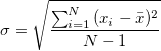
z-score: The z-score is the distance in standard deviation units for any given observation:

Empirical Rule or Three-Sigma Rule: Most of the data points fall within three standard deviations, with 68% would lie within 1 sd, 95% within 2 sd and 99.7% would fall within 3 sd.
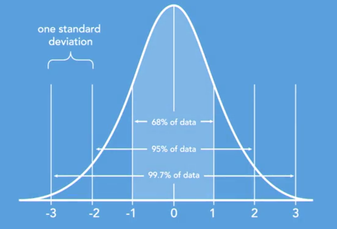
Note: It only works for symmetrically distributed data
Percentile Score: The percentile score for any value x in the dataset is given by:
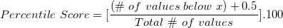
Probabilities
Event: An event is a set of probabilities e.g. When rolling a dice, an event A = (4,2,6) represents the event that an even number will appear.
Sample Space: All possible outcomes for a particular random experiment constitute it’s sample space.
Probability: The number of favorable outcomes divided by the number of all possible outcomes in a given situation.
Types of Probabilities
-
Classical Probability: The flipping of a coin is an example of classical probability because it is known that there are two sides to it and the likelihood of any one of them turning up is 50%. Objective Probabilities are based on calculations and classical probability is a type of Objective Probability.
-
Empirical Probability: The probabilities are the ones that are based on previously known data. For instance, Messi scoring more than ten goals in this season of FIFA is an example of Empirical probability because it is calculated on the basis of Messi’s previous record. This too is an example of Objective Probability since it’s also based on calculations.
-
Subjective Probability: These probabilities are not based on mathematical calculations and people use their opinions, their experiences to assert their viewpoints with some amount of relevant data that makes their own point stronger.
Addition Rule: The addition rule in probabilities is a rule that ensures that an event is not counted twice when calculating probabilities (where P(overlap) is the probability of both E1 and E2 occurring:

Conditional Probability: The probability of occurrence of an event given that some other event has already occurred.
Independent Events: If the probability of two events are completely unrelated. If we can prove that the probability of two occurring together is equal to the product of their individual probabilities, then we can say that the two events are independent.
Random Variable: The result of an experiment that has random outcomes is called a random variable. They can be of two types:
- Discrete RV: The number of drinks a person will order at Tank is an example of discrete random variable because it has to be a whole number.
- Continuous RV: The waiting time in line before one can order at a Burger King is an example of continuous variable because there are no fixed values that could be outcomes. The possibilities are infinite and continuous.
- Binomial RV: When an event has only two possible outcomes, the result is called a Binomial Random Variable.
Probability Density: The curves that represent the distribution of probabilities are called Probability Density curves.
Sampling
There are a few conditions that need to be considered before sampling is done from various sources:
- Size to Cost ratio: The appropriate size of the sample based upon the cost per data point in the sample
- Inherent Bias: If any bias was knowingly/unknowingly introduced while creating the sample, it will need to be considered!
- Quality of Sample
A simple random sample is the gold standard when collecting samples. This means, that any given point during the sample selection process, any individual has the same probability of being chosen as any other individual.
Some alternative sampling methods are:
- kth point: The first data point is selected and then every kth data point is selected in this method.
- Opportunity Sampling: The first n values are selected from the total data.
- Stratified Sampling: The whole sample is broken out into homogenous groups. Then we select few samples from each strata.
- Cluster Sampling: The whole sample is collected from heterogenous groups with data points with different characteristics. Then we select few samples from each group.
Confidence Intervals
As the name suggests, the confidence intervals present a level of confidence for a given interval.
Hypothesis Testing
The process to be able to test a hypothesis that has been presented.
Visualization Tips
- Tables: Useful for detailed recording and sharing of actual data
- Frequency Table: Displays the frequency of each observation in the data set
- Dot Plots: When you want to convey information that is discrete and individual to each observation.
- Histograms: When you want to convey frequencies of grouped bins, this could be useful.
- Pie Charts: Relative Frequency distributions are best represented with Pie Charts. They are also useful for representing distributions among qualitative variables where histograms wouldn’t be a very good measure.
Key Points
Types of Data
Overview
Teaching: min
Exercises: minQuestions
Cross-Sectional Data
It consists of variables, that are either quantitative or qualitative for a lot of different observations (usually called ‘cases’) and are taken from some defined population. All the cases are registered at a single point in time, or a reasonably short period of time. The techniques commonly used for this kind of data are ‘t-tests’ analysis of variance or regression depending on the kind and number of variables that are there in the data. It is noteworthy that each observation of a given variable or each set of variables are independent of every other observation in the dataset. The independence of the variables is a critical assumption when modelling cross-sectional data.
It is called cross-sectional data because we are measuring a cross-section of a defined population at a particular point in time or a very short period in time.
Time Series Data
If measurement on variables are taken over or through time. Every variable in a time series dataset is measured at equally spaced time intervals. Usually, the observations are not independent of each other in this case. Time series data can be classified into two types other thank the univariate and multivariate distinction and they are discussed in the time series chapter.
Key Points
Random Variables and Event Probabilities
Overview
Teaching: min
Exercises: minQuestions
Objectives
Random Variables and Event Probabilities
Random variables
Let \(Y\) be the result of a fair coin flip. Not a general coin flip, but a specific instance of flipping a specific coin at a specific time. Defined this way, \(Y\) is what’s known as a random variable, meaning a variable that takes on different values with different probabilities.^[Random variables are conventionally written using upper-case letters to distinguish them from ordinary mathematical variables which are bound to single values and conventionally written using lower-case letters.]
Probabilities are scaled between 0% and 100% as in natural language. If a coin flip is fair, there is a 50% chance the coin lands face up (“heads”) and a 50% chance it lands face down (“tails”). For concreteness and ease of analysis, random variables will be restricted to numerical values. For the specific coin flip in question, the random variable \(Y\) will take on the value 1 if the coin lands heads and the value 0 if it lands tails.
Events and probability
An outcome such as the coin landing heads is called an event in probability theory. For our purposes, events will be defined as conditions on random variables. For example, \(Y = 1\) denotes the event in which our coin flip lands heads. The functional \(\mbox{Pr}[\, \cdot \,]\) defines the probability of an event. For example, for our fair coin toss, the probability of the event of the coin landing heads is written as
[\mbox{Pr}[Y = 1] = 0.5.]
In order for the flip to be fair, we must have \(\mbox{Pr}[Y = 0] = 0.5\), too. The two events \(Y = 1\) and \(Y = 0\) are mutually exclusive in the sense that both of them cannot occur at the same time. In probabilistic notation,
[\mbox{Pr}[Y = 1 \ \mbox{and} \ Y = 0] = 0.]
The events \(Y = 1\) and \(Y = 0\) are also exhaustive, in the sense that at least one of them must occur. In probabilistic notation,
[\mbox{Pr}[Y = 1 \ \mbox{or} \ Y = 0] = 1.]
In these cases, events are conjoined (with “and”) and disjoined (with “or”). These operations apply in general to events, as does negation. As an example of negation,
[\mbox{Pr}[Y \neq 1] = 0.5.]
Sample spaces and possible worlds
Even though the coin flip will have a specific outcome in the real world, we consider alternative ways the world could have been. Thus even if the coin lands heads \((Y = 1)\), we entertain the possibility that it could’ve landed tails \((Y = 0)\). Such counterfactual reasoning is the key to understanding probability theory and applied statistical inference.
An alternative way the world could be, that is, a possible world, will determine the value of every random variable. The collection of all such possible worlds is called the sample space.^[The sample space conventionally written as \(\Omega\), the capitalized form of the last letter in the Greek alphabet.] The sample space may be conceptualized as an urn containing a ball for each possible way the world can be. On each ball is written the value of every random variable.^[Formally, a random variable \(X\) can be represented as a function from the sample space to a real value, i.e., \(X: \Omega \rightarrow \mathbb{R}\).
For each possible world \(\omega \in \Omega\), the variable \(X\) takes on a specific value
\(X(\omega) \in \mathbb{R}\).]
Statistic is the logic of uncertainty.
A sample space is the set of all possible outcomes of an experiment
An event is a subset of sample space
Now consider the event \(Y = 0\), in which our coin flip lands tails. In some worlds, the event occurs (i.e., \(0\) is the value recorded for \(Y\)) and in others it doesn’t. An event picks out the subset of worlds in which it occurs.^[Formally, an event is defined by a subset of the sample space, \(E \subseteq \Omega\).]
Naive definetion of probability
P(A) = #favorable outcome / #possible outcomes
Example: tossing of fair coins
Assumes all outcome equally likely, finite sample space
Sampling table
choose k objects out of n
| order matter | order doesn’t | |
|---|---|---|
| replace | n^k^ | \(\binom{n+k-1}{k}\) |
| don’t replace | n(n-1)…(n-k+1) | \(\binom{n}{k}\) |
- Don’t lose common sense
- Do check answers, especially by doing simple and extreme cases
- Label people , objects etc. If have n people, then label them 1,2…n
Example: 10 people, split into them of 6, team of 4 => \(\binom{10}{6}\) 2 teams of 5 => \(\binom{10}{5}\) /2
Problem: pick k times from set of n objects, where order doesn’t matter, with replacement.
Extreme cases: k = 0; k = 1; n = 2
Equiv : how many ways are there to put k indistinguishable particles into n distinguishable boxes?
Axioms of Probability
Non-naive definition
Probability sample consists of S and P, where S is sample space, and P , a function which takes an event \(A\subseteq S\) as input, returns \(P(A) \in [0,1]\) as output.
such that
- \(P(\phi) = 0, P(S) = 1\)\
- \(P(U_{n=1}^{\infty}A_n) = \sum_{n=1}^{\infty} P(A_n)\) if \(A1,A2..An\) are disjoint (not overlap)
Birthday Problem
(Exclude Feb 29, assume 365 days equally likely, assume indep. of birth)
k people , find prob. that two have same birthday
If k > 365, prob. is 1
Let k <= 365, \(P(no match) =\frac{ 365 * 364 *... (365 - k + 1) }{365^k}\)
P(match) ~ 50.7%, if k = 23; 97% if k = 50; 99.9999%, if k = 100
\(\binom{k}{2} = \frac{k(k-1)}{2}\) \(\binom{23}{2} = 253\)
Properties of Probability
- \(P(A^c) = 1 - P(A)\)\
- If \(A \subseteq B\) , then \(P(A) \subseteq P(B)\)\
- \[P(A\cup B) = P(A) + P(B) - P(A\cap B)\]
[P(A\cup B\cup C) = P(A) + P(B) + P(C) - P(A\cap B) - P(A\cap C) - P(B\cap C) + P(A\cap B\cap C)]
Proof:
- \(1 = P(S) = P(A\cap A^c) = P(A) + P(A^c)\)\
- \(B = A\cup(B\cap A^c)\) \(P(B) = P(A)+P(B\cap A^c)\)\
- \[P(A\cup B) = P(A\cap (B\cap A^c)) = P(A) + P(B\cap A^c)\]
General case:
deMontmort’s Problem(1713)
n cards labeled 1 to n, flipping cards over one by one, you win if the card that you name is the card that appears.
Let \(A_j\) be the event, ‘‘jth card matches”
\(P(A_j) = 1 / n\) since all position equally likely for card labeled j\
\(P(A_1\cap A_2) = (n-2)! / n! = 1/n(n-1)\)\
…
\(P(A_1\cap … A_k) = (n-k)! / n!\)\
\(P(A_1\cup …A_n) = n*1/n - n(n-1)/2 * 1/n(n-1) + …\)\
\(= 1 - 1/2! + 1/3! - 1/4! … (-1)^n1/n!\) \(\approx 1- 1/e\)
Story proof- proof by interpretation
Ex1 \(\binom{n}{k}\) = \(\binom{n}{n-k}\)
Ex2 n\(\binom{n-1}{k-1}\) = k\(\binom{n}{k}\) pick k people out of n, with one desigenate as president.
Ex3 \(\binom{m+n}{k} = \sum_{j=0}^k \binom{m}{j} \binom{n}{k-j}\) (vandermonde)
Simulating random variables
We are now going to turn our attention to computation, and in particular, simulation, with which we will use to estimate event probabilities.
The primitive unit of simulation is a function that acts like a random number generator. But we only have computers to work with and they are deterministic. At best, we can created so-called pseudorandom number generators. Pseudorandom number generators, if they are well coded, produce deterministic streams of output that appear to be random.^[There is a large literature on pseudorandom number generators and tests for measurable differences from truly random streams.]
For the time being, we will assume we have a primitive pseudorandom
number generator uniform_01_rng(), which behaves roughly like it has
a 50% chance of returning 1 and a 50% chance of returning 0.^[The name
arises because random variables in which every possible outcome is
equally likely are said to be uniform.]
Suppose we want to simulate our random variable \(Y\). We can do so by
calling uniform_01_rng and noting the answer.
A simple program to generate a realization of a random coin flip,
assign it to an integer variable y, and print the result could be
coded as follows.^[Computer programs are presented using a consistent
pseudocode, which provides a sketch of a program that should be
precise enough to be coded in a concrete programming language. R
implementations of the pseudocode generate the results and are
available in the source code repository for this book.]
import random

y = random.randint(0, 1)
print("y =", y)
The variable y is declared to be an integer and assigned to the
result of calling the uniform_01_rng() function.^[The use of a
lower-case \(y\) was not accidental. The variable \(y\) represents an
integer, which is the type of a realization of a random \(Y\)
representing the outcome of a coin flip. In code, variables are
written in typewriter font (e.g., y), whereas in text they are
written in italics like other mathematical variables (e.g., \(y\)).]
The print statement outputs the quoted string y = followed
by the value of the variable y. Executing the program might produce
the following output.
y = 1
If we run it a nine more times, it might print
for i in range(9):
    y = random.randint(0,1)
    print("y =", y)
y = 0
y = 1
y = 0
y = 1
y = 1
y = 0
y = 1
y = 1
y = 0
When we say it might print these things, we mean the results will depend on the state of the pseudorandom number generator.
Seeding a simulation
Simulations can be made exactly reproducible by setting what is known as the seed of a pseudorandom number generator. This seed establishes the deterministic sequence of results that the pseudorandom number generator produces. For instance, contrast the program
random.seed(1234)
for n in range(10):
    print(random.randint(0, 1)')
for n in range(10):
    print(random.randint(0, 1))
which produces the output
1 0 1 1 0 1 0 0 0 0
0 0 0 1 0 1 1 1 0 0
with the program
random.seed(1234)
for n in range(10):
    print(random.randint(0, 1)')
random.seed(1234)
for n in range(10):
    print(random.randint(0, 1))
which produces
1 0 0 0 0 0 0 1 0 0
1 0 0 0 0 0 0 1 0 0
Resetting the seed in the second case causes exactly the same ten pseudorandom numbers to be generated a second time. Every well-written pseudorandom number generator and piece of simulation code should allow the seed to be set manually to ensure reproducibility of results.^[Replicability of results with different seeds is a desirable, but stricter condition.]
Using simulation to estimate event probabilities
We know that \(\mbox{Pr}[Y = 1]\) is 0.5 because it represents the flip of a fair coin. Simulation based methods allow us to estimate event probabilities straightforwardly if we can generate random realizations of the random variables involved in the event definitions.
For example, we know we can generate multiple simulations of flipping the same coin. That is, we’re not simulating the result of flipping the same coin ten different times, but simulating ten different realizations of exactly the same random variable, which represents a single coin flip.
The fundamental method of computing event probabilities will not change as we move through this book. We simply simulate a sequence of values and return the proportion in which the event occurs as our estimate.
For example, let’s simulate 10 values of \(Y\) again and record the proportion of the simulated values that are 1. That is, we count the number of time the event occurs in that the simulated value \(y^{(m)}\) is equal to 1.
M = 100  # Set the value of M
occur = 0

for m in range(1, M+1):
    y = random.uniform(0, 1)
    occur += (y == 1)

estimate = occur / M
print(f"estimated Pr[Y = 1] = {estimate}")
The equality operator is written as ==, as in the condition y[m] ==
1 to distinguish it from the assignment statement y[m] = 1, which
sets the value of y[m] to 1. The condition expression y[m] == 1
evaluates to 1 if the condition is true and 0 otherwise.
If we let uniform_01_rng(M) be the result of generating M
pseudorandom coin flip results, the program can be shortened to
M = 100  # Set the value of M
y = [random.uniform(0, 1) for i in range(M)]
occur = sum([1 for i in y if i == 1])
estimate = occur / M
print(f"estimated Pr[Y = 1] = {estimate}")
A condition such as y == 1 on a sequence returns a sequence of the
same length with value 1 in positions where the condition is true. For
instance, if
y = (2, 1, 4, 2, 2, 1)
then
y == 2
evaluates to
(1, 0, 0, 1, 1, 0).
Thus sum(y == 1) is the number of positions in the sequence y
which have the value 1. Running the program provides the following
estimate based on ten simulation draws.
import numpy as np

M = 10
y_sim = np.random.binomial(1, 0.5, M)
for n in range(M):
    print(y_sim[n], end=' ')
print(f"estimated Pr[Y = 1] = {np.sum(y_sim) / M}")
Let’s try that a few more times.
M = 10

for k in range(1, 11):
    y_sim = np.random.binomial(1, 0.5, M)
    for n in range(M):
        print(y_sim[n], end=' ')
    print(f"estimated Pr[Y = 1] = {np.sum(y_sim) / M}")
1 1 0 0 0 1 1 1 0 0 estimated Pr[Y = 1] = 0.5
0 0 1 1 1 1 0 0 1 0 estimated Pr[Y = 1] = 0.5
0 0 0 1 1 0 1 0 1 1 estimated Pr[Y = 1] = 0.5
1 0 0 1 0 0 1 0 1 0 estimated Pr[Y = 1] = 0.4
1 1 0 0 1 0 0 0 0 1 estimated Pr[Y = 1] = 0.4
0 0 1 0 1 1 1 1 1 0 estimated Pr[Y = 1] = 0.6
1 1 0 1 1 1 0 0 0 1 estimated Pr[Y = 1] = 0.6
0 0 0 1 1 1 0 1 0 1 estimated Pr[Y = 1] = 0.5
0 0 0 0 1 0 1 0 0 1 estimated Pr[Y = 1] = 0.3
0 1 0 1 1 1 0 1 1 0 estimated Pr[Y = 1] = 0.6
The estimates are close, but not very exact. What if we use 100 simulations?
M = 100
y_sim = np.random.binomial(1, 0.5, M)
for n in range(M):
    print(y_sim[n], end=' ')
print(f"estimated Pr[Y = 1] = {np.sum(y_sim) / M}")
0 0 0 0 0 1 0 0 0 0 1 0 0 1 1 0 0 0 1 1 0 0 1 1 1 1 0 1 1 1 0 0 0 0 1 0 0 0 1 0 0 0 0 1 1 1 1 0 1 0 1 1 0 1 0 1 0 0 0 1 0 1 1 1 1 1 0 0 0 1 1 0 0 1 0 0 1 1 1 1 1 1 1 1 0 0 1 0 1 1 0 0 1 1 1 1 0 0 0 0
estimated Pr[Y = 1] = 0.48
That’s closer than most of the estimates based on ten simulation draws. Let’s try that a few more times without bothering to print all 100 simulated values,
for k in range(1, 11):
    y_sim = np.random.binomial(1, 0.5, M)
    print(f"estimated Pr[Y = 1] = {np.sum(y_sim) / M}")
estimated Pr[Y = 1] = 0.52
estimated Pr[Y = 1] = 0.58
estimated Pr[Y = 1] = 0.55
estimated Pr[Y = 1] = 0.37
estimated Pr[Y = 1] = 0.52
estimated Pr[Y = 1] = 0.48
estimated Pr[Y = 1] = 0.53
estimated Pr[Y = 1] = 0.53
estimated Pr[Y = 1] = 0.5
estimated Pr[Y = 1] = 0.53
What happens if we let \(M = 10,000\) simulations?
M = 10000

for k in range(1, 11):
    y_sim = np.random.binomial(1, 0.5, M)
    print(f"estimated Pr[Y = 1] = {np.sum(y_sim) / M}")
estimated Pr[Y = 1] = 0.5074
estimated Pr[Y = 1] = 0.4991
estimated Pr[Y = 1] = 0.5088
estimated Pr[Y = 1] = 0.5015
estimated Pr[Y = 1] = 0.4926
estimated Pr[Y = 1] = 0.4987
estimated Pr[Y = 1] = 0.4959
estimated Pr[Y = 1] = 0.5004
estimated Pr[Y = 1] = 0.4928
estimated Pr[Y = 1] = 0.5032
Now the estimates are very close to the true probability being estimated (i.e., 0.5, because the flip is fair). This raises the questions of how many simulation draws we need in order to be confident our estimates are close to the values being estimated.
Law of large numbers
Visualization in the form of simple plots goes a long way toward understanding concepts in statistics and probability. A traditional way to plot what happens as the number of simulation draws \(M\) increases is to keep a running tally of the estimate as each draw is made and plot the estimated event probability \(\mbox{Pr}[Y = 1]\) for each \(m \in 1:M\).^[See, for example, the quite wonderful little book, Bulmer, M.G., 1965. Principles of Statistics. Oliver and Boyd, Edinburgh.]
To calculate such a running tally of the estimate at each online, we can do this:
M = 100
y = np.zeros(M)
estimate = np.zeros(M)
occur = 0

for m in range(1, M+1):
    y[m-1] = np.random.randint(0, 2)
    occur += (y[m-1] == 1)
    estimate[m-1] = occur / m
    print(f"estimated Pr[Y = 1] after {m} trials = {estimate[m-1]}")
estimated Pr[Y = 1] after 1 trials = 0.0
estimated Pr[Y = 1] after 2 trials = 0.5
estimated Pr[Y = 1] after 3 trials = 0.3333333333333333
estimated Pr[Y = 1] after 4 trials = 0.25
estimated Pr[Y = 1] after 5 trials = 0.2
estimated Pr[Y = 1] after 6 trials = 0.3333333333333333
estimated Pr[Y = 1] after 7 trials = 0.42857142857142855
estimated Pr[Y = 1] after 8 trials = 0.375
estimated Pr[Y = 1] after 9 trials = 0.4444444444444444
estimated Pr[Y = 1] after 10 trials = 0.4
estimated Pr[Y = 1] after 11 trials = 0.36363636363636365
estimated Pr[Y = 1] after 12 trials = 0.3333333333333333
estimated Pr[Y = 1] after 13 trials = 0.3076923076923077
estimated Pr[Y = 1] after 14 trials = 0.2857142857142857
estimated Pr[Y = 1] after 15 trials = 0.3333333333333333
estimated Pr[Y = 1] after 16 trials = 0.375
estimated Pr[Y = 1] after 17 trials = 0.35294117647058826
estimated Pr[Y = 1] after 18 trials = 0.3888888888888889
estimated Pr[Y = 1] after 19 trials = 0.42105263157894735
estimated Pr[Y = 1] after 20 trials = 0.4
estimated Pr[Y = 1] after 21 trials = 0.42857142857142855
estimated Pr[Y = 1] after 22 trials = 0.45454545454545453
estimated Pr[Y = 1] after 23 trials = 0.43478260869565216
estimated Pr[Y = 1] after 24 trials = 0.4166666666666667
estimated Pr[Y = 1] after 25 trials = 0.4
estimated Pr[Y = 1] after 26 trials = 0.4230769230769231
estimated Pr[Y = 1] after 27 trials = 0.4444444444444444
estimated Pr[Y = 1] after 28 trials = 0.42857142857142855
estimated Pr[Y = 1] after 29 trials = 0.41379310344827586
estimated Pr[Y = 1] after 30 trials = 0.4
estimated Pr[Y = 1] after 31 trials = 0.3870967741935484
estimated Pr[Y = 1] after 32 trials = 0.40625
estimated Pr[Y = 1] after 33 trials = 0.3939393939393939
estimated Pr[Y = 1] after 34 trials = 0.4117647058823529
estimated Pr[Y = 1] after 35 trials = 0.4
estimated Pr[Y = 1] after 36 trials = 0.3888888888888889
estimated Pr[Y = 1] after 37 trials = 0.3783783783783784
estimated Pr[Y = 1] after 38 trials = 0.39473684210526316
estimated Pr[Y = 1] after 39 trials = 0.41025641025641024
estimated Pr[Y = 1] after 40 trials = 0.425
estimated Pr[Y = 1] after 41 trials = 0.43902439024390244
estimated Pr[Y = 1] after 42 trials = 0.42857142857142855
estimated Pr[Y = 1] after 43 trials = 0.4186046511627907
estimated Pr[Y = 1] after 44 trials = 0.4090909090909091
estimated Pr[Y = 1] after 45 trials = 0.4
estimated Pr[Y = 1] after 46 trials = 0.391304347826087
estimated Pr[Y = 1] after 47 trials = 0.40425531914893614
estimated Pr[Y = 1] after 48 trials = 0.4166666666666667
estimated Pr[Y = 1] after 49 trials = 0.42857142857142855
estimated Pr[Y = 1] after 50 trials = 0.42
estimated Pr[Y = 1] after 51 trials = 0.43137254901960786
estimated Pr[Y = 1] after 52 trials = 0.4423076923076923
estimated Pr[Y = 1] after 53 trials = 0.4528301886792453
estimated Pr[Y = 1] after 54 trials = 0.46296296296296297
estimated Pr[Y = 1] after 55 trials = 0.4727272727272727
estimated Pr[Y = 1] after 56 trials = 0.48214285714285715
estimated Pr[Y = 1] after 57 trials = 0.47368421052631576
estimated Pr[Y = 1] after 58 trials = 0.4827586206896552
estimated Pr[Y = 1] after 59 trials = 0.4745762711864407
estimated Pr[Y = 1] after 60 trials = 0.4666666666666667
estimated Pr[Y = 1] after 61 trials = 0.47540983606557374
estimated Pr[Y = 1] after 62 trials = 0.46774193548387094
estimated Pr[Y = 1] after 63 trials = 0.47619047619047616
estimated Pr[Y = 1] after 64 trials = 0.46875
estimated Pr[Y = 1] after 65 trials = 0.46153846153846156
estimated Pr[Y = 1] after 66 trials = 0.4696969696969697
estimated Pr[Y = 1] after 67 trials = 0.47761194029850745
estimated Pr[Y = 1] after 68 trials = 0.4852941176470588
estimated Pr[Y = 1] after 69 trials = 0.4782608695652174
estimated Pr[Y = 1] after 70 trials = 0.4714285714285714
estimated Pr[Y = 1] after 71 trials = 0.4788732394366197
estimated Pr[Y = 1] after 72 trials = 0.4861111111111111
estimated Pr[Y = 1] after 73 trials = 0.4931506849315068
estimated Pr[Y = 1] after 74 trials = 0.5
estimated Pr[Y = 1] after 75 trials = 0.49333333333333335
estimated Pr[Y = 1] after 76 trials = 0.4868421052631579
estimated Pr[Y = 1] after 77 trials = 0.4935064935064935
estimated Pr[Y = 1] after 78 trials = 0.5
estimated Pr[Y = 1] after 79 trials = 0.5063291139240507
estimated Pr[Y = 1] after 80 trials = 0.5125
estimated Pr[Y = 1] after 81 trials = 0.5185185185185185
estimated Pr[Y = 1] after 82 trials = 0.5121951219512195
estimated Pr[Y = 1] after 83 trials = 0.5180722891566265
estimated Pr[Y = 1] after 84 trials = 0.5119047619047619
estimated Pr[Y = 1] after 85 trials = 0.5176470588235295
estimated Pr[Y = 1] after 86 trials = 0.5116279069767442
estimated Pr[Y = 1] after 87 trials = 0.5172413793103449
estimated Pr[Y = 1] after 88 trials = 0.5227272727272727
estimated Pr[Y = 1] after 89 trials = 0.5280898876404494
estimated Pr[Y = 1] after 90 trials = 0.5333333333333333
estimated Pr[Y = 1] after 91 trials = 0.5384615384615384
estimated Pr[Y = 1] after 92 trials = 0.5434782608695652
estimated Pr[Y = 1] after 93 trials = 0.5483870967741935
estimated Pr[Y = 1] after 94 trials = 0.5425531914893617
estimated Pr[Y = 1] after 95 trials = 0.5473684210526316
estimated Pr[Y = 1] after 96 trials = 0.5520833333333334
estimated Pr[Y = 1] after 97 trials = 0.5463917525773195
estimated Pr[Y = 1] after 98 trials = 0.5510204081632653
estimated Pr[Y = 1] after 99 trials = 0.5454545454545454
estimated Pr[Y = 1] after 100 trials = 0.54
Recall that the expression (y[m] == 1) evaluates to 1 if the
condition holds and 0 otherwise. The result of running the program is
that estimate[m] will hold the estimate \(\mbox{Pr}[Y = 1]\) after \(m\)
simulations. We can then plot the estimates as a function
of the number of draws using a line plot to display the trend.
import numpy as np
import pandas as pd
import matplotlib.pyplot as plt
import random

np.random.seed(0)

M = 100000
Ms = []
y_sim = [random.randint(0,1) for i in range(M)]
hat_E_Y = []
Ms = []

for i in range(51):
    Ms.append(min(M, 10 ** (i / 10)))
    hat_E_Y.append(np.mean(y_sim[:int(Ms[i])]))

df = pd.DataFrame({'M': Ms, 'hat_E_Y': hat_E_Y})
plot = plt.scatter(df['M'], df['hat_E_Y'])
plt.axhline(y=0.5, color='red')
plt.xscale('log')
plt.xlabel('simulation draws')
plt.ylabel('estimated Pr[Y = 1]')
plt.xlim((1, 100000))
plt.ylim((0, 1))
plt.xticks([1, 50000], ["1", "50,000"])#, "100,000"])
plt.show()
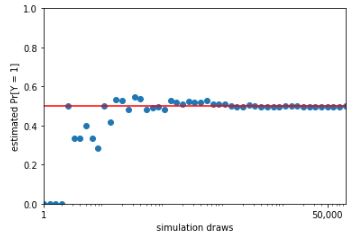
The linear scale of the previous plot obscures the behavior of the estimates. Consider instead a plot with the \(x\)-axis on the logarithmic scale.
Monte Carlo estimate of probability that a coin lands head as a function of the number of simulation draws. The line at 0.5 marks the true probability being estimated. The log-scaled \(x\)-axis makes the early rate of convergence more evident. Plotted on a linear scale, it is clear how quickly the estimates converge to roughly the right value.
import matplotlib.pyplot as plt
import pandas as pd

df = pd.DataFrame({'M': Ms, 'hat_E_Y': hat_E_Y})

plt.plot(df['M'], df['hat_E_Y'], linestyle='-', marker='o')
plt.axhline(y=0.5, color='red')
plt.xscale('log')
plt.xlabel('simulation draws')
plt.ylabel('estimated Pr[Y = 1]')
plt.xlim((1, 50000))
plt.ylim((0, 1))
plt.xticks([1, 50000], ["1", "50,000"])#, "100,000"])
plt.yticks([0, 0.25, 0.5, 0.75, 1.0])
plt.show()
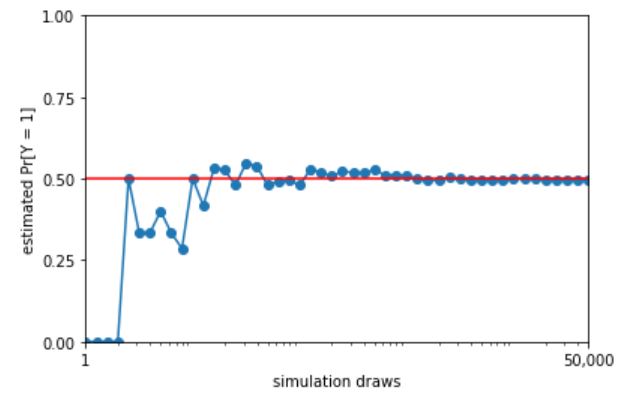
With a log-scaled \(x\)-axis, the values between 1 and 10 are plotted with the same width as the values between \(10\,000\) and \(100\,000\); both take up 20% of the width of the plot. On the linear scale, the values between 1 and 10 take up only \(\frac{10}{100\,000}\), or 0.01%, of the plot, whereas values between \(10\,000\) and \(100\,000\) take up 90% of the plot.
Plotting the progression of multiple simulations demonstrates the trend in errors.
Each of the one hundred grey lines represents the ratio of heads observed in a sequence of coin flips, the size of which indicated on the \(x\)-axis. The line at 0.5 indicates the probability a coin lands heads in a fair coin toss. The convergence of the ratio of heads to 0.5 in all of the sequences is clearly visible.
import numpy as np
import pandas as pd
import matplotlib.pyplot as plt
import seaborn as sns

np.random.seed(0)

M_max = 10000
J = 100
I = 47
N = I * J
df2 = pd.DataFrame({'r': [np.nan]*N, 'M': [np.nan]*N, 'hat_E_Y': [np.nan]*N})
pos = 0

for j in range(1, J+1):
    y_sim = np.random.binomial(1, 0.5, size=M_max)
    for i in range(4, 51):
        M = max(100, min(M_max, int((10**(1/10))**i)))
        hat_E_Y = np.mean(y_sim[:M])
        df2.loc[pos, :] = [j, M, hat_E_Y]
        pos += 1

pr_Y_eq_1_plot = sns.lineplot(data=df2, x='M', y='hat_E_Y', hue='r', alpha=0.15, linewidth=2)
pr_Y_eq_1_plot.axhline(y=0.5, color='red', linewidth=2)
pr_Y_eq_1_plot.set(xscale='log', xlabel='simulation draws', ylabel='estimated Pr[Y = 1]',
                    xlim=(100, 10000), ylim=(0.375, 0.625), xticks=[1000, 10000],
                    xticklabels=["1,000", "10,000"])
sns.set_theme(style='ticks')

plt.show()
Continuing where the previous plot left off, each of the one hundred grey lines represents the ratio of heads observed in a sequence of coin flips. The values on the \(x\) axis is one hundred times larger than in the previous plot, and the scale of the \(y\)-axis is one tenth as large. The trend in error reduction appears the same at the larger scale.
import numpy as np
import pandas as pd
import matplotlib.pyplot as plt
import seaborn as sns

np.random.seed(0)

M_max = 1000000
J = 100
I = 47
N = I * J
df2 = pd.DataFrame({'r': [np.nan]*N, 'M': [np.nan]*N, 'hat_E_Y': [np.nan]*N})
pos = 0

for j in range(1, J+1):
    y_sim = np.random.binomial(1, 0.5, size=M_max)
    for i in range(4, 61):
        M = max(100, min(M_max, int((10**(1/10))**i)))
        hat_E_Y = np.mean(y_sim[:M])
        df2.loc[pos, :] = [j, M, hat_E_Y]
        pos += 1

pr_Y_eq_1_plot = sns.lineplot(data=df2, x='M', y='hat_E_Y', hue='r', alpha=0.15)
pr_Y_eq_1_plot.axhline(y=0.5, color='red')
pr_Y_eq_1_plot.set(xscale='log', xlabel='simulation draws', ylabel='estimated Pr[Y = 1]',
                    xlim=(1e4, 1e6), ylim=(0.485, 0.515), xticks=[1e4, 1e5, 1e6],
                    xticklabels=["10,000", "100,000", "1,000,000"])
sns.set_theme(style='ticks')

plt.show()
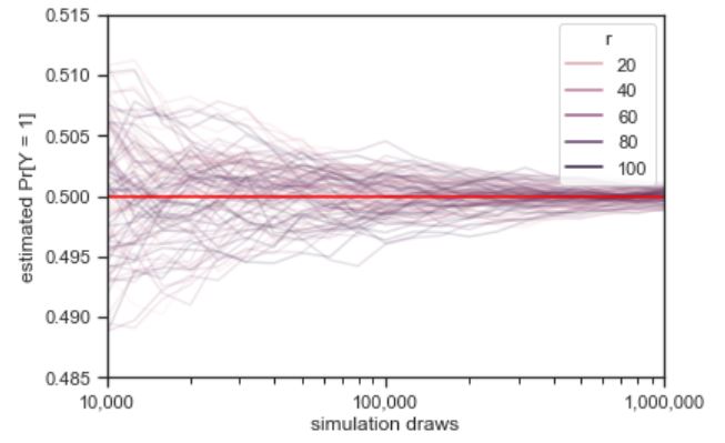
The law of large numbers^[Which technically comes in a strong and weak form.] says roughly that as the number of simulated values grows, the average will converge to the expected value. In this case, our estimate of \(\mbox{Pr}[Y = 1]\) can be seen to converge to the true value of 0.5 as the number of simulations \(M\) increases. Because the quantities involved are probabilistic, the exact specification is a little more subtle than the \(\epsilon\)-\(\delta\) proofs in calculus.
Simulation notation
We will use parenthesized superscripts to pick out the elements of a sequence of simulations. For example,
[y^{(1)}, y^{(2)}, \ldots, y^{(M)}]
will be used for \(M\) simulations of a single random variable \(Y\).^[Each \(y^{(m)}\) is a possible realization of \(Y\), which is why they are written using lowercase.] It’s important to keep in mind that this is \(M\) simulations of a single random variable, not a single simulation of \(M\) different random variables.
Before we get going, we’ll need to introduce indicator function notation. For example, we write
[\mathrm{I}[y^{(m)} = 1]
\begin{cases} 1 & \mbox{if} \ y^{(m)} = 1 \[4pt] 0 & \mbox{otherwise} \end{cases}]
The indicator function maps a condition, such as \(y^{(m)} = 1\) into the value 1 if the condition is true and 0 if it is false.^[Square bracket notation is used for functions when the argument is itself a function. For example, we write \(\mbox{Pr}[Y > 0]\) because \(Y\) is a random variable, which is modeled as a function. We also write \(\mathrm{I}[x^2 + y^2 = 1]\) because the standard bound variables \(x\) and \(y\) are functions from contexts defining variable values.]
Now we can write out the formula for our estimate of \(\mbox{Pr}[Y = 1]\) after \(M\) draws,
[\begin{array}{rcl} \mbox{Pr}[Y = 1] & \approx & \frac{\displaystyle \mathrm{I}[y^{(1)} = 1] \ + \ \mathrm{I}[y^{(2)} = 1] \ + \ \cdots \ + \ \mathrm{I}[y^{(M)} = 1]} {\displaystyle M} \end{array}]
That is, our estimate is the proportion of the simulated values which take on the value 1. It quickly becomes tedious to write out sequences, so we will use standard summation notation, where we write
[\mathrm{I}!\left[y^{(1)} = 1]
+ \mathrm{I}[y^{(2)} = 1]
+ \cdots
+ \mathrm{I}[y^{(M)} = 1\right]
\ =
\sum_{m=1}^M \mathrm{I}[y^{(m)} = 1]]
Thus we can write our simulation-based estimate of the probability that a fair coin flip lands heads as^[In general, the way to estimate an event probability \(\phi(Y)\) where \(\phi\) defines some condition, given simulations \(y^{(1)}, \ldots, y^{(M)}\) of \(Y\), is as \(\mbox{Pr}[\phi(Y)] = \frac{1}{M} \sum_{m = 1}^M \mathrm{I}[\phi(y^{(m)})].\)]
[\mbox{Pr}[Y = 1] \approx \frac{1}{M} \, \sum_{m=1}^M \mathrm{I}[y^{(m)} = 1]]
The form \(\frac{1}{M} \sum_{m=1}^M\) will recur repeatedly in simulation — it just says to average over values indexed by \(m \in 1:M\).^[We are finally in a position to state the strong law of large numbers as the event probability of a limit, \(\mbox{Pr}\!\left\lbrack \lim_{M \rightarrow \infty} \frac{1}{M} \sum_{m = 1}^M \mathrm{I}\!\left\lbrack y^{(m)} = 1 \right\rbrack \ = \ 0.5 \right\rbrack,\) where each \(y^{(m)}\) is a separate fair coin toss. ]
Central limit theorem
The law of large numbers tells us that with more simulations, our estimates become more and more accurate. But they do not tell us how quickly we can expect that convergence to proceed. The central limit theorem provides the convergence rate.
First, we have to be careful about what we’re defining. First, we define the error for an estimate as the difference from the true value,
[\left( \frac{1}{M} \sum_{m=1} \mathrm{I}[y^{(m)} = 1] \right) - 0.5]
The absolute error is just the absolute value^[In general, the absolute value function applied to a real number \(x\) is written as \(|x|\) and defined to be \(x\) if \(x\) is non-negative and \(-x\) if \(x\) is negative.] of this,
[\left| \, \left( \frac{1}{M} \sum_{m=1} \mathrm{I}[y^{(m)} = 1] \right) - 0.5 \, \right|]
The absolute error of the simulation-based probability estimate as a function of the number of simulation draws. One hundred sequences of one million flips are shown.
import numpy as np
import pandas as pd
import matplotlib.pyplot as plt
import seaborn as sns
from scipy.stats import binom

np.random.seed(1234)

M_max = 1000000
J = 100
I = 47
N = I * J

df2 = pd.DataFrame({'r': [np.nan]*N, 'M': [np.nan]*N, 'err_hat_E_Y': [np.nan]*N})
pos = 0

for j in range(1, J+1):
    y_sim = binom.rvs(1, 0.5, size=M_max)
    for i in range(4, 61):
        M = max(100, min(M_max, int((10**(1/10))**i)))
        err_hat_E_Y = abs(np.mean(y_sim[:M]) - 0.5)
        df2.loc[pos, :] = [j, M, err_hat_E_Y]
        pos += 1

abs_err_plot = sns.lineplot(data=df2, x='M', y='err_hat_E_Y', hue='r', alpha=0.15)
abs_err_plot.axhline(y=0.5, color='red')
abs_err_plot.set(xscale='log', xlabel='simulation draws', ylabel='absolute error',
                  xlim=(10000, 1000000), ylim=(0, 0.015),
                  xticks=[10000, 100000, 1000000], xticklabels=["10,000", "100,000", "1,000,000"])
sns.set_theme(style='ticks')

plt.show()
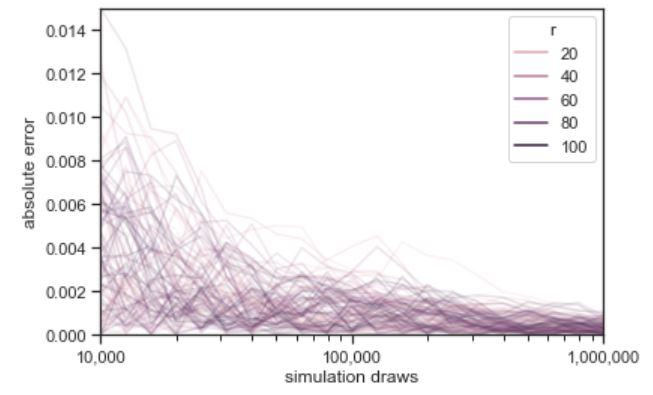
import numpy as np
from scipy.stats import norm

np.random.seed(1234)

M_max = int(1e6)
J = 300
Ms = 10 ** (np.arange(6, 13, 0.5) / 2)
N = len(Ms)
ys = np.empty((N, J))

for j in range(J):
    z = np.random.binomial(1, 0.5, M_max)
    for n in range(N):
        ys[n, j] = abs(np.mean(z[:int(Ms[n])]) - 0.5)

mean = np.empty(N)
sd = np.empty(N)
quant_68 = np.empty(N)
quant_95 = np.empty(N)

sixty_eight_pct = norm.cdf(1) - norm.cdf(-1)
ninety_five_pct = norm.cdf(2) - norm.cdf(-2)

for n in range(N):
    mean[n] = np.mean(ys[n, :])
    sd[n] = np.std(ys[n, :])
    quant_68[n] = np.quantile(ys[n, :], sixty_eight_pct)
    quant_95[n] = np.quantile(ys[n, :], ninety_five_pct)
Plotting both the number of simulations and the absolute error on the log scale reveals the rate at which the error decreases with more draws.
Absolute error versus number of simulation draws for 100 simulated sequences of \(M = 1,000,000\) draws. The blue line is at the 68 percent quantile and the red line at the 95 percent quantile of these draws. The relationship between the log number of draws and log error is revealed to be linear.
import numpy as np
from scipy.stats import binom, norm
import pandas as pd
import matplotlib.pyplot as plt
import math

np.random.seed(1234)

M_max = int(1e6)
J = 300
Ms = np.power(10, np.arange(6, 13, 0.5) / 2)
N = len(Ms)
ys = np.empty((N, J))
for j in range(J):
    z = np.random.binomial(1, 0.5, size=M_max)
    for n in range(N):
        ys[n, j] = np.abs(np.mean(z[:int(Ms[n])]) - 0.5)

mean = np.empty(N)
sd = np.empty(N)
quant_68 = np.empty(N)
quant_95 = np.empty(N)
sixty_eight_pct = norm.cdf(1) - norm.cdf(-1)
ninety_five_pct = norm.cdf(2) - norm.cdf(-2)
for n in range(N):
    mean[n] = np.mean(ys[n, :])
    sd[n] = np.std(ys[n, :], ddof=1)
    quant_68[n] = np.quantile(ys[n, :], q=sixty_eight_pct)
    quant_95[n] = np.quantile(ys[n, :], q=ninety_five_pct)

fudge = 1e-6
x = 0.5 * np.arange(1, 101)
log_abs_err_plot = plt.plot()
df2 = pd.DataFrame({'M': Ms, 'err_hat_E_Y': mean - 0.5})
for r in range(J):
    plt.plot(Ms, ys[:, r], alpha=0.15, color='gray')
plt.plot(Ms, quant_68, color='blue', linewidth=0.5)
plt.plot(Ms, quant_95, color='red', linewidth=0.5)
plt.xscale('log')
plt.xlim(0.9 * 1e3, 1.1 * 1e6)
plt.xticks([10**3, 10**4, 10**5, 10**6], ['1,000', '10,000', '100,000', '1,000,000'])
plt.ylim(0.8e-6, 2e-5)
plt.yticks([0.00005, 0.0005, 0.005, 0.05], ['0.00001', '0.0001', '0.001', '0.01'])
plt.xlabel('simulation draws')
plt.ylabel('log absolute error + 1e-5')
plt.show()
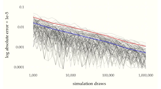
We can read two points \((x_1, y_1)\) and \((x_2, y_2)\) off of the graph for \(x_1 = 10\,000\) and \(x_2 = 100\,000\) as
print("x[1], y[1] = %7.f, %6.5f\nx[2], y[2] = %7.f, %6.5f" % (
        Ms[3], quant_68[3],
        Ms[5], quant_68[5]))
x[1], y[1] =    5623, 0.00685
x[2], y[2] =   17783, 0.00411
which gives us the following values on the log scale
import math

print(f"log x[1], log y[1] = {math.log(Ms[3]):5.2f}, {math.log(quant_68[3]):4.2f}\nlog x[2], log y[2] = {math.log(Ms[5]):5.2f}, {math.log(quant_68[5]):4.2f}")
log x[1], log y[1] =  8.63, -4.98
log x[2], log y[2] =  9.79, -5.49
Using the log scale values, the estimated slope of the reduction in quantile bounds is
print(f"estimated slope\n(log y[2] - log y[1])\n / (log x[2] - log x[1]) = {(math.log(quant_68[5]) - math.log(quant_68[3])) / (math.log(Ms[5]) - math.log(Ms[3])) :3.2f}")
estimated slope
(log y[2] - log y[1])
 / (log x[2] - log x[1])  =  -0.44
If we let \(\epsilon_M\) be the value of one of the quantile lines at \(M\) simulation draws, the linear relationship plotted in the figures have the form^[A line through the points \((x_1, y_1)\) and \((x_2, y_2)\) has \(\mbox{slope} = \frac{y_2 - y_1}{x_2 - x_1}.\)]
[\log \epsilon_M = -\frac{1}{2} \, \log M + \mbox{const}.]
When writing “const” in a mathematical expression, the presumption is that it refers to a constant that does not depend on the free variables of interest (here, \(M\), the number of simulation draws). Ignoring constants lets us focus on the order of the dependency. The red line and blue line have the same slope, but different constants.
Seeing how this plays out on the linear scale requires exponentiating both sides of the equation and reducing,
[\begin{array}{rcl} \exp(\log \epsilon_M) & = & \exp( -\frac{1}{2} \, \log M + \mbox{const} ) \[6pt] % \epsilon_M & = & \exp( -\frac{1}{2} \, \log M ) \times \exp(\mbox{const}) % \[6pt] \epsilon_M & = & \exp( \log M )^{-\frac{1}{2}} \times \exp(\mbox{const}) \[6pt] \epsilon_M & = & \exp(\mbox{const}) \times M^{-\frac{1}{2}} \end{array}]
Dropping the constant, this relationship between the expected absolute error \(\epsilon_M\) after \(M\) simulation draws may be succinctly summarized using proportionality notation,^[In general, we write \(f(x) \propto g(x)\) if there is a positive constant \(c\) that does not depend on \(x\) such that \(f(x) = c \times g(x).\) For example, \(3x^2 \propto 9x^2,\) with \(c = \frac{1}{3}\).]
[\displaystyle
\epsilon_M
\ \propto
\frac{\displaystyle 1}{\displaystyle \sqrt{M}}.]
This is a fundamental result in statistics derived from the central limit theorem. The central limit theorem governs the accuracy of almost all simulation-based estimates. We will return to a proper formulation when we have the scaffolding in place to deal with the pesky constant term.
In practice, what does this mean? It means that if we want to get an extra decimal place of accuracy in our estimates, we need one hundred (100) times as many draws. For example, the plot shows error rates bounded by roughly 0.01 with \(10\,000\) draws, yielding estimates that are very likely to be within \((0.49, 0.51).\) To reduce that likely error bound to 0.001, that is, ensuring estimates are very likely in \((0.0499, 0.501),\) requires 100 times as many draws (i.e., a whopping \(1\,000\,000\) draws).^[For some perspective, \(10\,000\) is the number of at bats in an entire twenty-year career for a baseball player, the number of field goal attempts in an entire career of most basketball players, and the size of a very large disease study or meta-analysis in epidemiology.]
Usually, one hundred draws will provide a good enough estimate of most quantities of interest in applied statistics. The variability of the estimate based on a single draw depends on the variability of the quantity being estimated. One hundred draws reduces the expected estimation bound to one tenth of the variability of a single draw. Reducing that variability to one hundredth of the variability of a single draw would require ten thousand draws. In most applications, the extra estimation accuracy is not worth the extra computation.
Exercise
1. A motorist encounters four consecutive traffic lights, each equally likely to be red or green. Let Z be the number of green lights passed by the motorist before being stopped by a red light. What is the probability distribution of Z?
Solution
Thinking of this problem as 4 buckets each with 2 possibilities paves a clear way to the solution of the problem. There are \(2^4 = 16\) possibilities. There is only one way for them to all be green (\(\xi = 4\)), and again only one way for 3 greens followed by one red (\(\xi = 3\)). Once you have get to \(\xi = 2\), then the last light can be either green or red giving two possibilities then at \(\xi = 1\) you have two lights that can be either red or green giving 4 possibilities. Clearly, then, there are 8 for the case of \(\xi = 0\). \(P(\xi) = \left\{ \begin{array}{rl} \frac{1}{2}, \xi=0 \\ \frac{1}{4}, \xi=1 \\ \frac{1}{8}, \xi=2 \\ \frac{1}{16}, \xi=3 \\ \frac{1}{16}, \xi=4 \end{array} \right. \label{answer4.1}\)
2. Give an example of two distinct random variables with the same distribution function.
Solution
To summarize what we want here: \(\begin{aligned} \xi_1 \neq \xi_2 \\ \Phi_{\xi_1}(x) = \Phi_{\xi_2}(x) \\ \int_{-\infty}^x p_{\xi_1}(x')dx' = \int_{-\infty}^x p_{\xi_2}(x')dx'\end{aligned}\) Since the question does not rule out the possibility that the probability distributions are the same, we can just say that \(\xi_1\) is the outcome of a coin-flip experiment and that \(\xi_2\) is the outcome of the first spin measurement of an EPR experiment.
4. A random variable \(\xi\) has probability density \(p_{\xi}(x) = \frac{a}{x^2 + 1} (-\infty < x <\infty)\). Find
a) The constant a;
b) The distribution function of \(\xi\);
c) The probability \(P{-1 < \xi < 1}\).Solution
The distribution is clearly not normalized so the first step will be to normalise it. \(\int^{\infty}_{-\infty} \frac{a}{x^2+1}dx = 1 = a \pi\)
\(a = \frac{1}{\pi}\)
Just by definition:
\(\Phi(x) = \int_{x}^{\infty} \frac{1}{\pi(x'^2+1)}dx' = \frac{\arctan x'}{\pi} \bigg|_{-\infty}^x\)
\(= \frac{\arctan x}{\pi}+\frac{1}{2}\) and last but not least:
\(P(\{-1 \leq x \leq 1\}) = \int_{-1}^1 \frac{1}{\pi(x'^2+1)} dx' = \frac{1}{2}\)
###
Solution
Once again we start by normalizing \(1= \int^{\infty}_{0} a x^2 e^{-k x} dx = -\left \frac{e^{-k x} \left(2+2 k x+k^2 x^2\right)}{k^3} \right]^{\infty}_{0}= \frac{2 a}{k^3}\) \(a = \frac{k^3}{2} \label{answer4.5a}\) \(\Phi(x) = \int^{x}_{0} \frac{k^3}{2}x'^2 e^{-k x'}dx' = 1 - \frac{e^{-k x} \left(2+2 k x+k^2 x^2\right)}{2} \label{answer4.5b}\) \(P( \{ 0 \leq x \leq \frac{1}{k} \} = \int_{0}^{\frac{1}{k}} \frac{k^3}{2}x^2 e^{-k x}dx = \frac{2e - 5}{2 e} \label{answer4.4c}\)
###
Solution
\(\Phi(\infty) = 1 \Rightarrow 1 = a + \frac{b \pi}{2}\) \(\Phi(-\infty) = 0 \Rightarrow 0 = a - \frac{b \pi}{2}\) Which you can solve to get \(\begin{aligned} b = \frac{1}{\pi} \\ a = \frac{1}{2}\end{aligned}\) Since \(\Phi\) is the integral of \(p\), we can take the derivative of it and then make sure it’s normalized. \(p(x) = \frac{d \Phi}{dx} = \frac{1}{2 \pi \left(1+\frac{x^2}{4}\right)}\) And the normalization is indeed still correct!
###
Solution
The area of the table is simply \(\pi R^2\) and the are of each of the smaller circles are \(\pi r^2\). The ratio of the sum of the area of the two circles to the total table area will be the chance that one of the circles gets hit: \(p = \frac{2r^2}{R^2}\).
###
Solution
Just like in example 2 in the book, this problem will go by very well if we draw a picture indicating the given criteria:
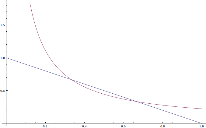 {width=”\textwidth”}
Where does this come from? \(\begin{aligned} x_1 + x_2 \leq 1 \\ x_2 \leq 1 - x_1\end{aligned}\) which is the straight line. \(\begin{aligned} x_1x_2 \leq \frac{2}{9} \\ x_2 \leq \frac{2}{9 x_1}\end{aligned}\) A little bit of algebra shows that these two lines intersect at \(\frac{1}{3}\) and \(\frac{2}{3}\) so the area underneath the straight line but not above the curved line is \(\begin{aligned} A =\int_0^{\frac{1}{3}}(1-x)dx + \int_{\frac{1}{3}}^{\frac{2}{3}}\frac{2}{9x}dx + \int_{\frac{2}{3}}^{1}(1-x)dx \\ = \frac{5}{18} + \int_{\frac{1}{3}}^{\frac{2}{3}}\frac{2}{9x}dx + \frac{1}{18} \\ = \frac{1}{3} + \int_{\frac{1}{3}}^{\frac{2}{3}}\frac{2}{9x}dx \\ = \frac{1}{3 } + \frac{2 \ln 2}{9} \approx 0.487366\end{aligned}\) And the answer is properly normalized since the initial probability distributions were unity (the box length is only 1).
###
Solution
As we showed in example number 4, \(p_{\eta}\) is the convolution of \(p_{\xi_1}\) and \(p_{\xi_2}\). \(\begin{aligned} p_{\eta}(y) = \int_{-\infty}^{\infty} p_{\xi_1}(y-x)p_{\xi_2}(x)dx\end{aligned}\) I think the integration will look more logical if we stick in Heaviside step-functions. \(\begin{aligned} p_{\eta}(y) = \frac{1}{6} \int_{-\infty}^{\infty}e^{-\frac{y-x}{3}}e^{-\frac{x}{3}}H(y-x)H(x)dx\end{aligned}\) Clearly \(x\) has to be greater than zero and \(y\) must be greater than x, leading to the following limits of integration. \(\begin{aligned} p_{\eta}(y) = \frac{1}{6} \int_{0}^{y}e^{-\frac{y-x}{3}}e^{-\frac{x}{3}}dx \\ = e^{-\frac{y}{3}}\left(1- e^{-\frac{y}{6}} \right)\end{aligned}\) Only when y is greater than zero!
###
Solution
Due to the magic of addition, finding the probability distribution of \(\xi_1 + \xi_2 + \xi_3\) is no different than the probability distribution of \((\xi_1 + \xi_2) + \xi_3\) but we already know what the probability distribtution of the parenthesized quantity is: \(p_{\xi_1 + \xi_2}(y) = \int_{-\infty}^{\infty} p_{\xi_1}(y-x)p_{\xi_2}(x)dx\) Therefore the total combination is \(p_{\xi_1 + \xi_2+ \xi_3}(z) = \int_{-\infty}^{\infty} p_{\xi_1 + \xi_2}(z-y)p_{\xi_3}(y)dx\) \(p_{\xi_1 + \xi_2+ \xi_3}(z) = \int_{-\infty}^{\infty} \left[ \int_{-\infty}^{\infty} p_{\xi_1}(z-y-x)p_{\xi_2}(x)dx \right]p_{\xi_3}(y)dy\) \(p_{\xi_1 + \xi_2+ \xi_3}(z) = \int_{-\infty}^{\infty} \int_{-\infty}^{\infty} p_{\xi_1}(z-y-x)p_{\xi_2}(x)p_{\xi_3}(y)dx dy\) which is just a triple convolution.
###
Solution
\(p_{\xi}(n) = \frac{1}{3^n}\) therefore \(\textbf{E}\xi = \sum_{n=1}^{\infty}\frac{n}{3^n} = \frac{3}{4} \label{answer4.11}\)
###
Since finding a ball in one urn versus the other urn has nothing to do with each other, the events are clearly independent so we can multiply probabilities. The probability of finding a white ball at any given urn is \(p_w = \frac{w}{w+b}\) If you find a white ball on the \(n^{th}\) try then that means you found \(n-1\) black balls before you got to the white ball. \(p_w(n) = \frac{b^{n-1} w}{(w+b)^n}\) \(\textbf{E}n = \sum_{i=1}^{\infty}n p_w(n) = \sum_{i=1}^{\infty}n \frac{b^{n-1} w}{(w+b)^n} = \frac{b+w}{w}\) Which is the total number of balls drawn, subtract one to get the average number of black balls drawn: \(m=\frac{b}{w}\) Now for the variance. to start with we need the average of the square of the random variable. \(\textbf{E}n^2 = \sum_{i=1}^{\infty}n^2 p_w(n) = \sum_{i=1}^{\infty}n^2 \frac{b^{n-1} w}{(w+b)^n} = \frac{(b+w) (2 b+w)}{w^2}\) \(\textbf{D}n = \textbf{E}n^2 - (\textbf{E}n)^2 = \frac{(b+w) (2 b+w)}{w^2} - \left( \frac{b+w}{w} \right)^2 = \frac{b^2+wb}{w^2}\) A note that we don’t need to subtract anything for the variance since shifting a distribution over does not affect its variance: just its average.
###
Solution
\(\textbf{E}\xi = \int_{-\infty}^{\infty} x\frac{1}{2}e^{-|x|} = 0\) because the function is even about \(x=0\). \(\textbf{E}\xi^2 = \int_{-\infty}^{\infty} x^2\frac{1}{2}e^{-|x|} = 2\) Therefore: \(\textbf{D}\xi = \textbf{E}\xi^2 - (\textbf{E}\xi)^2 = 2\)
###
Solution
\(\textbf{E}x = \int_{a-b}^{a+b} \frac{xdx}{2b} = a\) \(\textbf{E}x^2 = \int_{a-b}^{a+b} \frac{x^2dx}{2b} = a^2+\frac{b^2}{3}\) Therefore: \(\textbf{D}x = \frac{b^2}{3}\)
###
Solution
If the distribution function is \(\Phi_{\xi}(x) = a + b \arcsin x, |x| \leq 1\) then it must fulfill the proper boundary conditions as specified by both the problem and the definition of a distribution function. \(\Phi_{\xi}(-1)= 0 = a - b \frac{\pi}{2}\) \(\Phi_{\xi}(1) = 1 = a + b \frac{\pi}{2}\) Some easy algebra gets you \(\begin{aligned} \Phi_{\xi}(x) = \frac{1}{2} + \frac{1}{\pi} \arcsin x\end{aligned}\) Therefore: \(p_{\xi}(x) = \frac{1}{\pi\sqrt{1-x^2}}\) \(\begin{aligned} \textbf{E}x = \int_{-1}^{1} \frac{x dx}{\pi\sqrt{1-x^2}} = 0 \\ \textbf{D}x = \int_{-1}^{1} \frac{x^2 dx}{\pi\sqrt{1-x^2}} = \frac{1}{2}\end{aligned}\)
###
Solution
Each side of the die has the same probability, \(\frac{1}{6}\) \(\textbf{E}x = \sum_{i=1}^6 \frac{i}{6} = \frac{7}{2}\) \(\textbf{E}x^2 = \sum_{i=1}^6 \frac{i^2}{6} = \frac{91}{6}\) Therefore: \(\textbf{D}x = \frac{91}{6} - \left( \frac{7}{2} \right)^2 = \frac{91}{6} - \frac{49}{4} = \frac{35}{12}\)
###
Solution
This problem may seem difficult until you realize that being \(\pm \frac{5}{2}\) away from the mean means you’re at either 1 or 6, meaning that there’s a unity probability of being that far from the mean. Chebyshev’s inequality, however, would have us believe that \(P \{ |x + \textbf{E}x| > \frac{5}{2} \} \leq \frac{4}{25} \frac{91}{6} = \frac{182}{75} = 2.42667\) which is not only far off from the actual answer, it’s also unphysical to have probabilities greater than 1!
###
Solution
We want to consider the probability distribution of \(\xi\) by way of \(\eta\) \(\eta = e^{\frac{a\xi}{2}}\) We know from Chebyshev’s identity:
\(P\{ \eta > \epsilon(\eta) \} \leq \frac{\textbf{E}\eta^2}{\epsilon(\eta)^2}\) Let \(\epsilon\) be the error in \(\xi\) we’re looking for. \(P\{ \xi > \epsilon \} \leq \frac{\textbf{E}(e^{\frac{a\xi}{2}})^2}{(e^{\frac{a\epsilon}{2}})^2}\) \(P\{ \xi > \epsilon \} \leq \frac{\textbf{E}e^{a\xi}}{e^{a\epsilon}}\)
###
Solution
First some initial calculations: \(\begin{aligned} \textbf{E}\xi = \frac{1}{4} \left( -2+-1+1+2 \right) = 0 \\ \textbf{E}\xi^2 = \frac{1}{4} \left( (-2)^2+(-1)^2+1^2+2^2 \right) = \frac{10}{4} = \frac{5}{2} = \textbf{E}\eta \\ \textbf{E}\xi^4 = \frac{1}{4} \left( (-2)^4+(-1)^4+1^4+2^4 \right) = \frac{34}{4} = \frac{17}{2} = \textbf{E}\eta^2\end{aligned}\) Now, we know that \(\begin{aligned} r = \frac{\textbf{E} \left[ (\xi - \textbf{E}\xi)(\eta - \textbf{E}\eta) \right]}{(\textbf{E}\xi^2 - (\textbf{E}\xi)^2)(\textbf{E}\eta^2 - (\textbf{E}\eta)^2)}\end{aligned}\) The denominator \(D\) is the easiest: \(D = \left( \frac{5}{2} - 0 \right)\left( \frac{17}{2} - \frac{5^2}{2^2} \right) = \frac{45}{8}\) Now for the numerator: \(\begin{aligned} \textbf{E} \left[ (\xi - \textbf{E}\xi)(\eta - \textbf{E}\eta) \right] \\ = \frac{1}{16} \left[ \sum_{\xi, \eta} (\xi - \textbf{E}\xi)(\eta - \textbf{E}\eta) \right]\end{aligned}\) If we look at the set we’ll be summing over, we have \({\xi - \textbf{E}\xi} = -2, -1, 1, 2\) and \({\eta - \textbf{E}\eta} = \frac{3}{2}, -\frac{3}{2}, -\frac{3}{2}, \frac{3}{2}\) and clearly, since we have to sum over all possible products, since both distributions are symmetric about 0, the sum will go to zero. \(r=0\)
###
Solution
First some initial calculations: \(\begin{aligned} \textbf{E}x_1 = \int_0^{\frac{\pi}{2}} x_1 \sin x_1 \sin x_2 dx_1dx_2 = 1 \\ \textbf{E}x_2 = 1 \\ \textbf{E}x_1^2 = \int_0^{\frac{\pi}{2}} x_1^2 \sin x_1 \sin x_2 dx_1dx_2 = (\pi - 2) \\ \textbf{E}x_2^2 = (\pi - 2) \\\end{aligned}\) \(\begin{aligned} \textbf{E} \left[ (x_1 - \textbf{E}x_1)(x_2 - \textbf{E}x_2) \right] \\ = \int_0^{\frac{\pi}{2}} \int_0^{\frac{\pi}{2}} \left[(x_1 - 1)(x_2 - 1)\right]\sin x_1 \sin x_2 dx_1dx_2 = 0 \\ \sigma_1 \sigma_2 = \sqrt{(\pi - 2)- 1}\sqrt{(\pi - 2) - 1} = (\pi - 3) \\ r= \frac{0}{(\pi - 3)} = 0\end{aligned}\)
###
Solution
First some initial calculations: \(\begin{aligned} \textbf{E}x_1 = \frac{1}{2}\int_0^{\frac{\pi}{2}} x_1 \sin (x_1 + x_2) dx_1dx_2 = \frac{\pi}{4} \\ \textbf{E}x_2 = \frac{\pi}{4} \\ \textbf{E}x_1^2 = \frac{1}{2}\int_0^{\frac{\pi}{2}} x_1^2 \sin (x_1 + x_2) dx_1dx_2 = -2+\frac{\pi}{2} +\frac{\pi ^2}{8} \\ \textbf{E}x_2^2 = -2+\frac{\pi}{2} +\frac{\pi ^2}{8} \\\end{aligned}\) \(\begin{aligned} \textbf{E} \left[ (x_1 - \textbf{E}x_1)(x_2 - \textbf{E}x_2) \right] \\ = \frac{1}{2}\int_0^{\frac{\pi}{2}} \int_0^{\frac{\pi}{2}} \sin (x_1 + x_2) \left[(x_1 - \frac{\pi}{2})(x_2 - \frac{\pi}{2})\right]dx_1dx_2 = -\frac{1}{16} (\pi -4)^2 \\ \sigma_1\sigma_2 = -2+\pi +\frac{\pi ^2}{2} +\frac{\pi^2}{8} - \frac{\pi^2}{16} = -2+\pi +\frac{\pi ^2}{2} +\frac{\pi^2}{16} \\ r = \frac{-\frac{1}{16} (\pi -4)^2}{-2+\pi +\frac{\pi ^2}{2} +\frac{\pi^2}{16}}\end{aligned}\)
###
Solution
\(\begin{aligned} E\xi = \int_{-\infty}^{\infty} \frac{x}{\pi(1+x^2)}dx = \left \frac{\log \left(x^2+1\right)}{2 \pi } \right]_{-\infty}^{\infty} \rightarrow \infty \\ E\xi^2 = \int_{-\infty}^{\infty} \frac{x^2}{\pi(1+x^2)}dx = \left \frac{x}{\pi }-\frac{\tan ^{-1}(x)}{\pi } \right]_{-\infty}^{\infty} \rightarrow \infty\end{aligned}\) Neither integral actually converges so we cannot define averages or dispersions for this distribution.
Key Points
Multiple Random Variables and Probability Functions
Overview
Teaching: min
Exercises: minQuestions
Objectives
Multiple Random Variables and Probability Functions
Multiple random variables
Random variables do not exist in isolation. We started with a single random variable \(Y\) representing the result of a single, specific coin flip. Suppose we fairly flip the coin three times? Then we can have random variables \(Y_1, Y_2, Y_3\) representing the results of each of the flips. We can assume each flip is independent in that it doesn’t depend on the result of other flips. Each of these variables \(Y_n\) for \(n \in 1:3\) has \(\mbox{Pr}[Y_n = 1] = 0.5\) and \(\mbox{Pr}[Y_n = 0] = 0.5\).
We can combine multiple random variables using arithmetic operations. We have already seen comparison operators in writing the event \(Y = 1\). If \(Y_1, \ldots, Y_{10}\) are random variables representing ten coin flips, then we can define their sum as
[Z = Y_1 + Y_2 + Y_3]
We can simulate values of \(Z\) by simulating values of \(Y_1, Y_2, Y_3\) and adding them.
from random import randint

y1 = randint(0, 1)
y2 = randint(0, 1)
y3 = randint(0, 1)
z = y1 + y2 + y3
print("z =", z)
z = 3
It is easier and less error prone to collapse similar values into arrays and operate on the arrays collectively, or with loops if necessary.
y = []
for n in range(1, 4):
    y.append(randint(0, 1))
z = sum(y)
print("z =", z)
Running this program a few times we get
z = 2
z = 3
z = 1
z = 3
z = 1
We can use simulation to evaluate the probability of an outcome that
combines multiple random variables. For example, to evaluate
\(\mbox{Pr}[Z = 2]\), we run the simulation many times and count the
proportion of results that are two.^[The sum is calculated using
notation \(sum(y[m, ])\),
which is defined to be
\(sum(y[m, ]) = y[m, 1] + ... + y[m, N],\) where N is the number of entries in row m of the variable y.]
M = 10000  # Define the value of M
y = [[randint(0, 1) for n in range(3)] for m in range(M)]  # Generate random integers and store them in a 2D list y
z = [sum(row) for row in y]  # Calculate the sum of each row in y and store them in a list z
Pr_is_two = sum(z == 2) / M  # Calculate the proportion of elements in z that are equal to 2
print("Pr_is_two =", Pr_is_two)
Pr_is_two = 0.3692
As in our other probability estimates, we simulate the variable of
interest \(Z\) a total of \(M\) times, yielding \(z^{(1)}, \ldots,
z^{(m)}\). Here, that requires simulating \(y_1^{(m)}, y_2^{(m)},
y_3^{(m)}\) and adding them for each \(z^{(m)}\). We then just count the
number of times Z is simulated to be equal to 2 and divide by the
number of simulations.
Letting \(M = 100,000\), and running five times, we get
import random
M = 10000  # Define the value of M
random.seed(1234)
for i in range(5):
    y = [[randint(0, 1) for n in range(3)] for m in range(M)]  # Generate random integers and store them in a 2D list y
    z = [sum(row) for row in y]  # Calculate the sum of each row in y and store them in a list z
    Pr_is_two = sum([1 for i in z if i == 2]) / M  # Calculate the proportion of elements in z that are equal to 2
    print("Pr_is_two =", Pr_is_two)
Pr_is_two = 0.3709
Pr_is_two = 0.3712
Pr_is_two = 0.3707
Pr_is_two = 0.3721
Pr_is_two = 0.3725
Nailing down that final digit is going to require one hundred times as many iterations (i.e, \(M = 10,000,000\) iterations). Let’s see what that looks like.
from numpy.random import binomial
M = 10000000

for k in range(1, 6):
    Z = binomial(3, 0.5, M)
    Pr_Z_is_2 = sum(Z == 2) / M
    print(f"Pr[Z == 2] = {Pr_Z_is_2:.3f}")
Pr[Z == 2] = 0.375
Pr[Z == 2] = 0.375
Pr[Z == 2] = 0.375
Pr[Z == 2] = 0.375
Pr[Z == 2] = 0.375
We can do the same for the other numbers, to get a complete picture of taking the probability of each number of heads in separate coin flips.
M = 10000000

for z in range(0, 4):
    Z = binomial(3, 0.5, M)
    Pr_Z_is_z = s
Pr[Z == 0] = 0.125
Pr[Z == 1] = 0.375
Pr[Z == 2] = 0.375
Pr[Z == 3] = 0.125
What if we flip four coins instead of three?
M = 10000000

for z in range(0, 5):
    Z = binomial(4, 0.5, M)
    Pr_Z_is_z = sum(Z == z) / M
    print(f"Pr[Z == {z}] = {Pr_Z_is_z:.3f}")
Pr[Z == 0] = 0.063
Pr[Z == 1] = 0.250
Pr[Z == 2] = 0.375
Pr[Z == 3] = 0.250
Pr[Z == 4] = 0.063
Discrete random variables
So far, we have only considered random numbers that take a finite number of integer values. A random variable that only takes values in the integers, i.e., values in
[\mathbb{Z} = \ldots -2, -1, 0, 1, 2, \ldots]
is said to be a discrete random variable.^[In general, any countable set of numerical values could be used as values of a discrete random variable. A set of values is countable if each of its members can be assigned a unique counting number in \(\mathbb{N} = 0, 1, 2, \ldots\). The integers \(\mathbb{Z}\) can be mapped to natural numbers \(\mathbb{N}\) by interleaving, \(\begin{array}{rcl}\mathbb{Z} & & \mathbb{N} \\ \hline 0 & \mapsto & 0 \\ -1 & \mapsto & 1 \\ 1 & \mapsto & 2 \\ -2 & \mapsto &3 \\ 2 & \mapsto & 4 \\ & \vdots & \end{array}\)]
Probability mass functions
It’s going to be convenient to have a function that maps each possible outcome in a variable to its probability. In general, this will be possible if and only if the variable is discrete, as defined in the previous section.
For example, if we reconsider \(Z = Y_1 + \cdots Y_4\), the number of heads in four separate coin flips, we can define a function^[We implicitly assume that functions return zero for arguments not listed.]
[\begin{array}{rclll}
p_Z(0) & = & 1/16 & & \mathrm{TTTT}
p_Z(1) & = & 4/16 & & \mathrm{HTTT, THTT, TTHT, TTTH}
p_Z(2) & = & 6/16 & & \mathrm{HHTT, HTHT, HTTH, THHT, THTH, TTTH}
p_Z(3) & = & 4/16 & & \mathrm{HHHT, HHTH, HTHH, THHH}
p_Z(4) & = & 1/16 & & \mathrm{HHHH}
\end{array}]
There are sixteen possible outcomes of flipping four coins. Because the flips are separate and fair, each possible outcome is equally likely. The sequences corresponding to each count of heads (i.e., value of \(Z\)) are recorded in the rightmost columns. The probabilities are derived by dividing the number of ways a value for \(Z\) can arise by the number of possible outcomes.
This function \(p_Z\) was constructed to map a value \(u\) for \(Z\) to the event probability that \(Z = u\),^[Conventionally, this is written as \(p_Z(z) = \mbox{Pr}[Z = z],\) but that can be confusing with upper case \(Z\) denoting a random variable and lower case \(z\) denoting an ordinary variable.]
[p_Z(u) = \mbox{Pr}[Z = u].]
A function defined as above is said to be the probability mass function of the random variable \(Z\). Every discrete random variable has a unique probability mass function.
Probability mass functions represent probabilities of a discrete set of outcomes. The sum of all such probabilities must be one because at least one of the outcomes must occur.^[More formally, if \(Y\) is a discrete random variable, then \(\sum_u \, p_Y(u) = 1,\) where the summation variable \(u\) ranges over all possible values of \(Y\). We are going to start writing this with the standard overloading of lower and upper case \(Y\) as \(\sum_y \, p_Y(y) = 1.\)]
With large numbers of counts based on simulation, we can more readily apprehend what is going on with a plot. Discrete simulations are typically plotted using bar plots, where the outcomes are arrayed on the \(x\) axis with a vertical bar over each one whose height is proportional to the frequency of that outcome.
Plot of \(M = 100,000\) simulations of the probability mass function of a random variable defined as the number of heads in ten specific coin flips.
import numpy as np
import matplotlib.pyplot as plt

np.random.seed(1234)

M = 100000
u = np.random.binomial(10, 0.5, M)
x = np.arange(0, 11)
y = np.zeros(11)

for n in range(0, 11):
    y[n] = np.sum(u == n)

plt.bar(x, y, color='#F8F8F0', edgecolor='black')
plt.xticks(np.arange(0, 11, 2), labels=['0', '2', '4', '6', '8', '10'])
plt.yticks(np.arange(0, 35000, 10000), labels=['0', '10000', '20000', '30000'])
plt.xlabel('Z')
plt.ylabel('count')
plt.show()
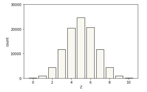
The actual frequencies are not relevant, only the relative sizes. A simple probability estimate from simulation provides a probability for each outcome proportional to its height.^[And proportional to its area because the bars are of equal width.]
This plot can easily be repeated to see what happens as the number of bins grows.
Plot of \(M = 1,000,000\) simulations of a variable \(Z\) representing the number of heads in \(N\) coin flips. Each plot represents a different \(N\). Because the bars are the same width and the \(x\) axes are scaled to the same range in all plots, the total length of all bars laid end to end is the same in each plot; similarly, the total area of the bars in each plot is the same.
import pandas as pd
import numpy as np
import matplotlib.pyplot as plt
import seaborn as sns

np.random.seed(1234)
df = pd.DataFrame()
for N in [5, 10, 15, 20, 25, 30]:
    M = 1000000
    u = np.random.binomial(N, 0.5, size=M)
    x = np.arange(N+1)
    y = np.array([np.sum(u==n) for n in x])
    df = df.append(pd.DataFrame({'N': np.repeat(N, N+1),
                                  'Z': x,
                                  'count': y}))

bar_plot = sns.catplot(data=df, x='Z', y='count', kind='bar',
                       col='N', col_wrap=3, palette='Blues_d')
bar_plot.set_axis_labels('Z', 'Count')
bar_plot.set_xticklabels([str(i) if i%10==0 else '' for i in x])
plt.show()
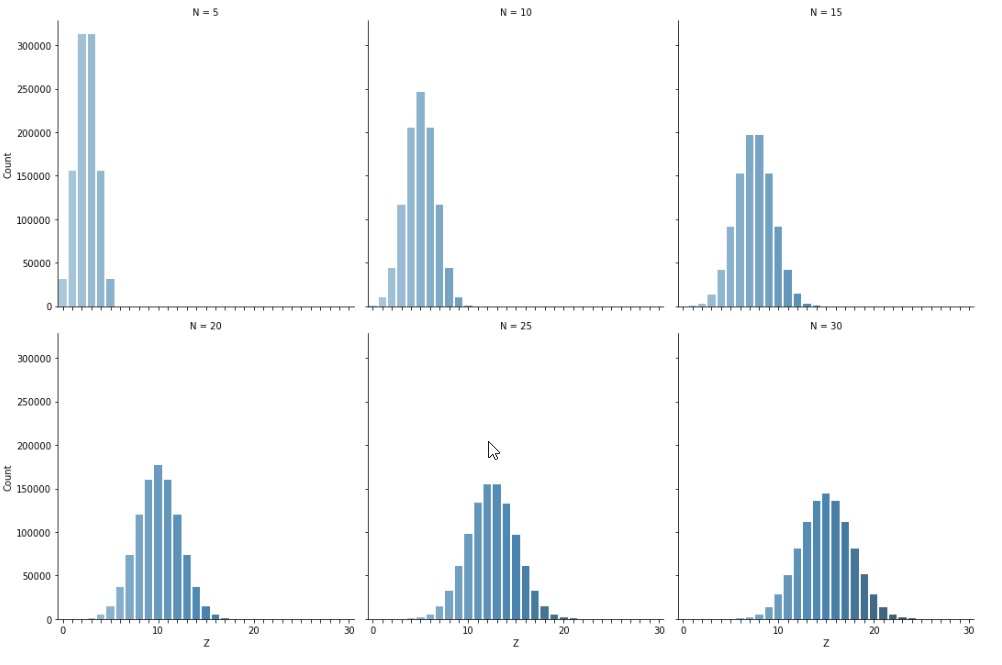
Dice
Let \(Y\) be a random variable representing a fair throw of a six-sided die. We can describe this variable easily through it’s probability mass function, which is uniform (i.e., assigns each possible outcome the same probability).
[p_Y(y) \ =
\begin{cases}
\frac{1}{6} & \mbox{if} \ y \in 1:6
\[4pt]
0 & \mbox{otherwise}
\end{cases}]
Games like Monopoly use a pair of six-sided dice and consider the sum of the results. That is, \(Y_1\) and \(Y_2\) are fair six-sided die rolls and \(Z = Y_1 + Y_2\) is the result. Games like Dungeons \& Dragons use a trio of six-sided dice and consider the sum of the results. In that scenario, \(Y_1, Y_2, Y_3\) are the results of fair six-sided die rolls and \(Z = Y_1 + Y_2 + Y_3\). Dungeons and Dragons also uses four six-sided die of which the best 3 are summed to produce a result. Let’s simulate some of these approaches and see what the results look like based on \(M = 100,0000\) simulations.^[The simulations are identical to before, only using 1:6 in the range of uniform variables.]
Estimated \(p_Y(y)\) for case of \(Y\) being the sum of three six-sided dice (3d6) or the sum of the highest three of four six-sided dice (3 of 4d6).
import numpy as np
import pandas as pd
from plotnine import *

M = 100000

three_d6 = np.random.randint(1, 7, size=M) + np.random.randint(1, 7, size=M) + np.random.randint(1, 7, size=M)

three_of_4d6 = np.zeros(M)
for m in range(M):
    rolls = np.sort(np.random.randint(1, 7, size=4))
    three_of_4d6[m] = np.sum(rolls[1:])

tot_3d6 = np.zeros(16)
tot_3_of_4d6 = np.zeros(16)
for n in range(3, 19):
    tot_3d6[n - 3] = np.sum(three_d6 == n)
    tot_3_of_4d6[n - 3] = np.sum(three_of_4d6 == n)

att_dice_df = pd.DataFrame({'probability': np.concatenate([tot_3d6 / M, tot_3_of_4d6 / M]),
'roll': np.concatenate([np.arange(3, 19), np.arange(3, 19)]),
'dice': np.concatenate([np.repeat('3d6', 16), np.repeat('3 of 4d6', 16)])})

att_dice_plot = (ggplot(att_dice_df, aes(x='roll', y='probability')) +
geom_bar(stat='identity', colour='black', fill='#F8F8F0') +
facet_wrap('dice', labeller=labeller(dice=label_both)) +
scale_x_continuous(name='y',
breaks=[3, 6, 9, 12, 15, 18],
labels=[3, 6, 9, 12, 15, 18]) +
scale_y_continuous(name="estimated " + "p[Y](y)") +
ggtitle("Distribution of 3d6 vs. 3 of 4d6 rolls") +
theme(panel_spacing=2.0))
att_dice_plot
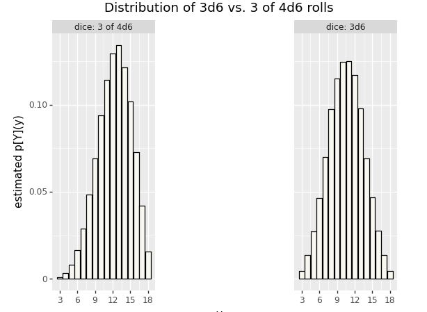
Dungeons and Dragons also uses 20-sided dice.^[In physical games, an icosahedral die is used. The icosahedron is a regular polyhedron with 20 equilateral triangular faces, giving it the largest number of faces among the five Platonic solids.] The fifth edition of the game introduced the notion of advantage, where two 20-sided dice are rolled and the higher result retained, as well as disadvantage, which retains the lower result of the two dice. Here’s a simulation using \(M = 100,000\). The counts are converted to estimated probabilities on the vertical axis in the usual way by dividing by \(M\).
Estimated \(p_Y(y)\) for case of \(Y\) being a single twenty-sided die (d20), the higher two twenty-sided die rolls (max 2d20), and the lower of two 20-sided die rolls (min 2d20).
import numpy as np
import pandas as pd
import matplotlib.pyplot as plt
import seaborn as sns

M = 100000
d20 = np.random.choice(20, size=M, replace=True)
max_2d20 = np.zeros(M)
min_2d20 = np.zeros(M)

for m in range(M):
    max_2d20[m] = max(np.random.choice(20, size=2, replace=True))
    min_2d20[m] = min(np.random.choice(20, size=2, replace=True))

tot_d20 = np.zeros(20)
tot_max_2d20 = np.zeros(20)
tot_min_2d20 = np.zeros(20)

for n in range(20):
    tot_d20[n] = sum(d20 == (n+1))
    tot_max_2d20[n] = sum(max_2d20 == (n+1))
    tot_min_2d20[n] = sum(min_2d20 == (n+1))

att_d20_df = pd.DataFrame({'probability': np.concatenate([tot_d20/M, tot_max_2d20/M, tot_min_2d20/M]),
                           'roll': np.concatenate([np.arange(1,21), np.arange(1,21), np.arange(1,21)]),
                           'dice': np.repeat(['1d20', 'max 2d20', 'min 2d20'], 20)})

# create a FacetGrid with 3 columns
g = sns.FacetGrid(att_d20_df, col='dice', col_wrap=3, height=4, aspect=1)

# plot each histogram using FacetGrid.map()
g.map(sns.barplot, 'roll', 'probability', color="blue")#F8F8F0")

# set x and y axis labels and titles
g.set_axis_labels('y', 'estimated $p_Y(y)$')
g.fig.subplots_adjust(top=0.9)
g.fig.suptitle('')

# set xticks for each plot
for ax in g.axes.flat:
    ax.set_xticks([0, 4, 9, 14, 19])
    ax.set_xticklabels([1, 5, 10, 15, 20])

plt.show()
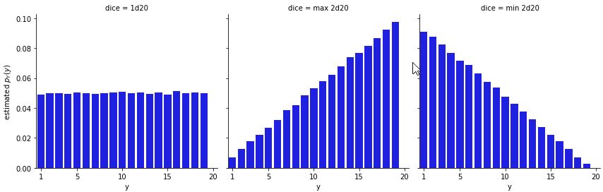
The most likely roll is a 20 when taking the best of two rolls and the most likely roll is 1 when taking the worst of two rolls.^[The chance for a 20 when taking the best of two 20-sided die rolls is \(1 - \left(\frac{19}{20}\right)^2 \approx 0.098\); the chance of rolling 1 is \(\left(\frac{1}{20}\right)^2 = 0.0025\). The probabilities are reversed when taking the worst of two 20-sided die rolls.] The min and max plots are mirror images of each other as is to be expected by the consecutive nature of the numbers and the min/max operations.
Spinners and the Bernoulli distribution
Some games, such as All Star Baseball, come with spinners rather than dice. The beauty of spinners is that they can be divided into two areas, one with a 27% chance of occurring in a fair spin and one with a 73% chance of occurring.^[27% is roughly the chance of a hit in an at bat.] Now suppose we have a random variable \(Y\) representing the result of a fair spin. Its probability mass function is
[p_Y(y)
\ =
\begin{cases}
0.27 & \mbox{if} \ \ y = 1
0.73 & \mbox{if} \ \ y = 0
\end{cases}]
To simplify our notation, we are going to start defining useful functions that can be used as probability mass functions. Our first example is the so-called Bernoulli^[Named after Jacob Bernoulli (1654–1705), one of several prominent mathematicians in the family.] distribution. We define it as a function with somewhat peculiar notation,
[\mathrm{Bernoulli}(y \mid \theta)
\ =
\begin{cases}
\theta & \mbox{if} \ \ y = 1
1 - \theta & \mbox{if} \ \ y = 0
\end{cases}]
The vertical bar (\(\mid\)) separates the variate argument \(y\), which we think of as an outcome, from the parameter argument \(\theta \in [0, 1]\), which determines the probability of the outcome. In this case, the variate \(y\) is discrete, and can take on only the values zero and one, so we write \(y \in 0:1\). The parameter \(\theta\), on the other hand, is continuous and can take on any value between zero and one (inclusive of endpoints), so we write \(y \in [0, 1]\).^[Interval notation \([0, 1]\) is used for the set of values \(x\) such that \(0 \leq x \leq 1\). Parentheses are used for exclusive endpoints, so that \((0, 1)\) is taken to be the set of \(x\) such that \(0 < x < 1\).]
This notation allows us to simplify our baseball example. Going back to our example random variable \(Y\) which had a 27% chance of being 1 and a 73% chance of being 0, we can write
[p_Y(y) = \mathrm{Bernoulli}(y \mid 0.27).]
To simplify notation even further, we will say that a random variable \(U\) has a Bernoulli distribution and write
[U \sim \mathrm{Bernoulli}(\theta)]
to indicate that the probability mass function of \(U\) is
[p_U(u) = \mathrm{Bernoulli}(u \mid \theta).]
Cumulative distribution functions
In Dungeons \& Dragons, the players are often concerned with probabilities of rolling higher than a given number (or equivalently, rolling lower than a given number. For example, they may need to roll a 15 to sneak by an orc. Such probabilities are conventionally given in the form of cumulative distribution functions. If \(Y\) is a random variable, its cumulative distribution function \(F_Y\) is defined by
[F_Y(y) = \mbox{Pr}[Y \leq y].]
The event probability on the right is calculated the same way as always in a simulation, by counting the number of simulated values in which the condition holds and dividing by the number of simulations.
We can plot the cumulative distribution function for the straight twenty-sided die roll and the rolls with advantage (best of two rolls) or disadvantage (worst of two rolls). Here’s the result using the same simulations as in the last plot, with \(M = 100,000\).
Cumulative distribution function for three variables corresponding to rolling a single 20-sided die, or rolling two 20-sided dice and taking the best or worst result.
import pandas as pd
import numpy as np
import matplotlib.pyplot as plt
import seaborn as sns

M = 100000
d20 = np.random.choice(20, size=M, replace=True)
max_2d20 = np.zeros(M)
min_2d20 = np.zeros(M)

for m in range(M):
    max_2d20[m] = max(np.random.choice(20, size=2, replace=True))
    min_2d20[m] = min(np.random.choice(20, size=2, replace=True))

tot_d20 = np.zeros(20)
tot_max_2d20 = np.zeros(20)
tot_min_2d20 = np.zeros(20)

for n in range(20):
    tot_d20[n] = np.sum(d20 == (n+1))
    tot_max_2d20[n] = np.sum(max_2d20 == (n+1))
    tot_min_2d20[n] = np.sum(min_2d20 == (n+1))

cum_d20 = np.cumsum(tot_d20)
cum_max_2d20 = np.cumsum(tot_max_2d20)
cum_min_2d20 = np.cumsum(tot_min_2d20)

cum_d20_df = pd.DataFrame({
    'probability': np.concatenate((cum_d20/M, cum_max_2d20/M, cum_min_2d20/M)),
    'roll': np.concatenate((np.arange(1, 21), np.arange(1, 21), np.arange(1, 21))),
    'dice': np.concatenate((np.repeat("1d20", 20), np.repeat("max 2d20", 20), np.repeat("min 2d20", 20)))
})

cum_d20_plot = (
    sns.relplot(data=cum_d20_df, x='roll', y='probability', kind='line', hue='dice',
                facet_kws={'margin_titles': True}, col='dice', col_wrap=3)
    .set(xlabel='y', xticks=[1, 5, 10, 15, 20],
         xticklabels=[1, 5, 10, 15, 20], ylabel=r'estimated $F_Y(y)$')
    .set_titles("{col_name}")
    .fig
)

plt.show()
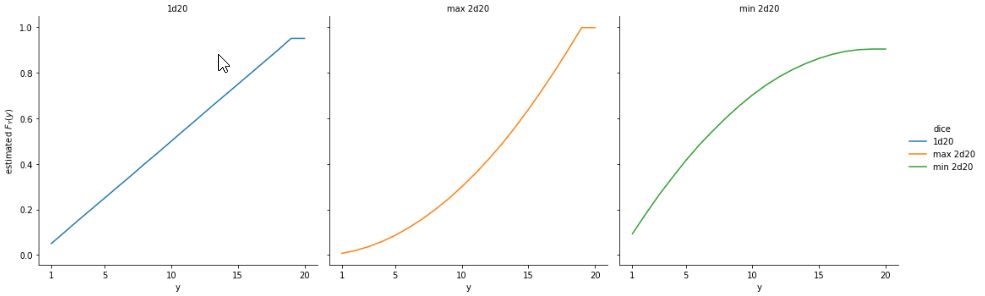
The plot is rendered as a point plot, though this isn’t quite sensible for discrete distributions—the intermediate values are not real. It’s easy to see that there’s a 50% chance of rolling 5 or lower in a single die throw; with the best of 2 it’s more like a 20% chance and with the worst of 2, it’s more like a 75% chance.
Usually in Dungeons \& Dragons, players care about rolling more than a given number, not less, or they’d have to be subtracting all the time. This is where the complementary cumulative distribution function comes in. For a random variable \(Y\), the complementary cumulative distribution function is
[F^{\complement}_Y(y) \ = \ 1 - F_Y(y) \ = \ \mbox{Pr}[Y > y].]
It’s easier to see with a plot how it relates to the usual cumulative distribution function.
Complementary cumulative distributions for a single 20-sided die, the best of two dice, and the worst of two dice.
import pandas as pd
import numpy as np
import matplotlib.pyplot as plt
import seaborn as sns

M = 100000
d20 = np.random.choice(20, size=M, replace=True)
max_2d20 = np.zeros(M)
min_2d20 = np.zeros(M)

for m in range(M):
    max_2d20[m] = max(np.random.choice(20, size=2, replace=True))
    min_2d20[m] = min(np.random.choice(20, size=2, replace=True))

tot_d20 = np.zeros(20)
tot_max_2d20 = np.zeros(20)
tot_min_2d20 = np.zeros(20)

for n in range(20):
    tot_d20[n] = np.sum(d20 == (n+1))
    tot_max_2d20[n] = np.sum(max_2d20 == (n+1))
    tot_min_2d20[n] = np.sum(min_2d20 == (n+1))

cum_d20 = np.cumsum(tot_d20)
cum_max_2d20 = np.cumsum(tot_max_2d20)
cum_min_2d20 = np.cumsum(tot_min_2d20)

ccum_d20_df = pd.DataFrame({
    'probability': np.concatenate((1 - cum_d20/M, 1 - cum_max_2d20/M, 1 - cum_min_2d20/M)),
    'roll': np.concatenate((np.arange(1, 21), np.arange(1, 21), np.arange(1, 21))),
    'dice': np.concatenate((np.repeat("1d20", 20), np.repeat("max 2d20", 20), np.repeat("min 2d20", 20)))
})

ccum_d20_plot = (
    sns.relplot(data=ccum_d20_df, x='roll', y='probability', kind='line', hue='dice',
                facet_kws={'margin_titles': True}, col='dice', col_wrap=3)
    .set(xlabel='y', xticks=[1, 5, 10, 15, 20],
         xticklabels=[1, 5, 10, 15, 20], ylabel=r'estimated $F_Y(y)$')
    .set_titles("{col_name}")
    .fig
)
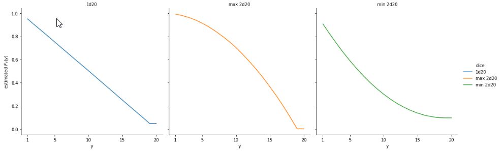
Infinite discrete random variables
Consider an experiment in which a coin is tossed until a heads appears. Let the random variable \(U\) be the number of tosses that came up tails before the first head comes up. The legal sequences are H (0 tails), TH (1 tails), TTH (2 tails), and so on. There is no upper limit to how many tails may appear before the first heads.
Here’s some code to create \(M\) simulations of the variable \(U\).^[This
code uses a while loop, which repeats as long as its condition
evaluates to true (i.e., 1). Here, the condition compares the output
of the random number generator directly rather than assigning to an
intermediate value. We have also introduced the increment operator
+=, which adds the value of the right hand side to the variable on
the left hand side.]
import random

M = 10 # replace with the desired value of M
u = [0] * M

for m in range(M):
    while random.randint(0, 1) == 0:
        u[m] += 1
This looks dangerous! The body of a while-loop (here u[m] + 1) is
executed iteratively as long as the condition is true.^[If we write
while (1 + 1 == 2) we produce what is known as an infinite loop,
i.e., one that never terminates.] Shouldn’t we be worried that the
random number generator will just continue to throw tails (i.e., 0)
so that the program never terminates?^[The answer is “yes,” in general,
because programmers are error prone.] In this case, no, because the
odds are vanishingly small that \(U\) gets large. For example,
[\begin{array}{rcl} \mbox{Pr}[U < 10] & = & p_U(0) + p_U(1) + \cdots p_U(9) \[6pt] & = & \frac{1}{2} + \cdots + \frac{1}{1024} \[6pt] & \approx & 0.999. \end{array}]
Going further, \(\mbox{Pr}[U < 20] \approx 0.999\,999\), and so on. So there’s not much chance of running very long at all, much less forever.
With the concern of non-termination out of the way, let’s see what we get with \(M = 50\) simulations of \(U\).
import random

def sim_u():
    u = 0
    while random.randint(0, 1) == 0:
        u += 1
    return u

random.seed(1234)
for m1 in range(1, 6):
    for m2 in range(1, 11):
        print(f"{sim_u():4d}", end="")
    print()
0	6	4	0	0	5	2	3	1	0
0	0	2	3	1	0	3	5	2	0
1	0	2	1	1	1	0	0	0	0
0	1	1	0	0	0	2	0	2	0
0	1	2	1	0	2	2	3	0	0
It’s very hard to discern a pattern here. There are a lot of zero values, but also some large values. For cases like these, we can use a bar plot to plot the values. This time, we’re going to use \(M = 10,000\) to get a better picture of the pattern.
Frequency of outcomes in \(10,000\) simulation draws of \(U\), the number of tails seen before a head in a coin-tossing experiment.
import random
import numpy as np
import matplotlib.pyplot as plt
import seaborn as sns

def sim_u():
    u = 0
    while random.randint(0, 1) == 0:
        u += 1
    return u

random.seed(1234)
M = 10000
u = np.array([sim_u() for m in range(M)])
x = np.arange(max(u) + 1)
y = np.array([np.sum(u == n) for n in range(max(u) + 1)])

bar_plot = sns.barplot(x=x, y=y, color="blue")#F8F8F0")
bar_plot.set(xlabel="U", ylabel="count")
bar_plot.set(xticks=np.arange(13), xticklabels=np.arange(13))
bar_plot.set(yticks=[1000, 2000, 3000, 4000, 5000], yticklabels=[1000, 2000, 3000, 4000, 5000])
plt.show()
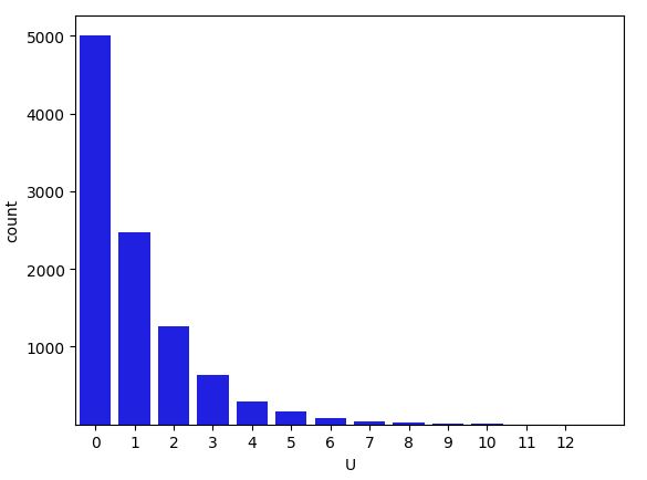
The \(x\)-axis represents the value of \(U\) and the \(y\)-axis the number of times that value arose in the simulation.^[Despite \(U\) having infinitely many possible values, it will only take on finitely many of them in a finite sample.] Each additional throw of tails appears to cut the probability of occurrence in half result seems to have about half the probability of the previous one. This is what we should expect because each coin toss brings a 50% probability of a tails result. This exponential decay^[Exponential decay means each additional outcome is only a fraction as likely as the previous one.] in the counts with the number of tails thrown is more obvious when plotted on the log scale.
Frequency of outcomes in \(10,000\) simulation draws of \(U\), the number of tails seen before a head in a coin-tossing experiment, this time with the outcome count on the log scale to illustrate the exponentially decreasing probabilities of each successive number of tails.
import random
import numpy as np
import matplotlib.pyplot as plt
import seaborn as sns

def sim_u():
    u = 0
    while random.randint(0, 1) == 0:
        u += 1
    return u

random.seed('1234')
M = 10000
u = np.array([sim_u() for m in range(M)])
x = np.arange(max(u) + 1)
y = np.array([np.sum(u == n) for n in range(max(u) + 1)])

log_bar_plot = sns.barplot(x=x, y=y, color="blue")#F8F8F0")
log_bar_plot.set(xlabel="U", ylabel="count")
log_bar_plot.set(xticks=np.arange(13), xticklabels=np.arange(13))
log_bar_plot.set(yticks=[8, 40, 200, 1000, 5000], yticklabels=[8, 40, 200, 1000, 5000])
log_bar_plot.set(yscale="log")
plt.show()
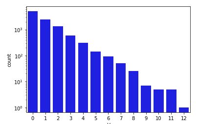
There is a 50% probability that the first toss is heads, yielding a sequence of zero tails, and \(U = 0\). Each successive number of tails is half as likely as the previous, because another tail will have to be thrown, which has a 50% probability.^[In symbols, \(\mbox{Pr}[U = n + 1] \ = \ \frac{1}{2} \mbox{Pr}[U = n].\) ]
Thus the overall probability mass function for \(U\) is^[An elementary result of calculus is that \(\sum_{n = 0}^{\infty} \frac{1}{2^{n + 1}} \ = \ \frac{1}{2} + \frac{1}{4} + \frac{1}{8} + \frac{1}{16} + \cdots \ = \ 1.\)]
[\begin{array}{rclcl}
p_U(0) & = & \frac{1}{2} & = & \frac{1}{2}
p_U(1) & = & \frac{1}{2} \times \frac{1}{2} & = & \frac{1}{4}
p_U(2) & = & \frac{1}{2} \times \frac{1}{2} \times \frac{1}{2} & = & \frac{1}{8}
& \vdots &
p_U(u) & = & \underbrace{\frac{1}{2} \times
\cdots \times \frac{1}{2}}_{u + 1 \ \mathrm{times}}
& = &
\left( \frac{1}{2} \right)^{u + 1}
& \vdots &
\end{array}]
Even though there are infinitely many possible realizations of the random variable \(U\), simulation may still be used to compute event probabilities, such as \(\mbox{Pr}[U \leq 3]\), by
M = 10000
u = np.array([sim_u() for m in range(M)])
leq3 = np.array([u[m] <= 3 for m in range(M)])

print('est Pr[U <= 3] =', sum(leq3) / M)
Let’s see what we get with \(M = 100,000\),
est Pr[U <= 3] = 0.9394
Writing out the analytic answer involves an infinite sum,
[\mbox{Pr}[U \leq 3]
\ =
\sum_{u = 0}^{\infty} p_U(u) \mathrm{I}[u \leq 3].]
We can recognize that all of the terms where \(u > 3\) are zero, so that this reduces to
[\begin{array}{rcl} \mbox{Pr}[U \leq 3] & = & p_U(0) + p_U(1) + p_U(2) + p_U(3) \[8pt] & = & \frac{1}{2}
- \frac{1}{4}
- \frac{1}{8}
- \frac{1}{16} \[8pt] & \approx & 0.938. \end{array}]
Simulation is not that clever. It just blindly simulates values of \(u\), many of which turn out to be larger than three. In the sequence of simulated values, many were larger than three—the histogram summarized a much larger simulation, none of the values of which were that large.
Given that we only ever run a finite number of iterations and thus only ever see a finite number of values, how does simulation get the right answer?^[Spoiler alert! The technical answer, like so much in statistics, is that the central limit theorem kicks in.] Isn’t there some kind of bias from only visiting smallish values? The answer is “no” precisely because the values that are not simulated are so rare. Their total probability mass, when added together is small, so they cannot have much influence on the simulated answer. For simulations to get the right answer,^[Given some qualifications!] they need only visit the typical values seen in simulation, not the extreme values.^[The sparsity problem grows exponentially worse in higher dimensions and uncountably worse with continuous random variables.]
The Chevalier de Méré’s challenge
Antoine Gombaud, the Chevalier de Méré,^[Self appointed!] challenged Blaise Pascal to explain how it was possible that the probability of throwing at least one six in four throws of a single six-sided die is slightly greater than \(\frac{1}{2}\), whereas the probability of throwing two sixes in 24 throws of a pair of six-sided die was slightly less than \(\frac{1}{2}\).^[Smith, D. A., 1929. A Source Book on Mathematics. McGraw-Hill, New York; cited in Bulmer, 1967, p. 26.] We can evaluate these claims by simulation directly.^[Working out the example analytically, there is a \(\frac{35}{36}\) chance of not throwing double six with two six-sided dice, and so \(\left( \frac{35}{36} \right)^{24}\) is the probability of not throwing at least one double six in 24 throws, and so \(1 - \left( \frac{35}{36} \right)^{24} \approx 0.491\) is the probability of throwing at least one double-six in 24 fair throws of a pair of six-sided dice.]
To represent the problem in probabilistic notation, we introduce a random variable \(Y_{1, k} \in 1:6\) and \(Y_{2, k} \in 1:6\) for each of the two dice in each of the \(k \in 1:24\) throws. Define the outcome of the game as the random variable
[Z \ =
\begin{cases}
1 \ \ \mbox{if there is a} \ k \ \mbox{such that} \ Y_{1,k} = Y_{2,k} = 6,
\ \mbox{and}
\[4pt]
0 \ \ \mbox{otherwise}
\end{cases}]
That is, \(Z = 1\) if there is at least one double-six in the 24 throws. The Chevalier de Méré was inquiring about the value of the event probability \(\mbox{Pr}[Z = 1]\), i.e., the chance of winning by throwing at least one double six in 24 fair throws of a pair of dice.
We will introduce variables for the full range of simulated random
variable values and simulation indexes in the following program.^[The
simulation indexes use parentheses rather than the traditional
brackets and come first so that, e.g., the simulated value y(m) will
consist of a \(2 \times 24\) collection of values, matching the size of
\(Y\).]
M = 10000
success = np.zeros(M, dtype=bool)

for m in range(M):
    y = np.zeros((2, 24))
    z = np.zeros(24)

    for k in range(24):
        y[0, k] = np.random.randint(1, 7)
        y[1, k] = np.random.randint(1, 7)
        z[k] = y[0, k] + y[1, k]

    success[m] = np.sum(z == 12) > 0

print('Pr[double-six in 24 throws] =', np.sum(success) / M)
Let’s run that for \(M = 100,000\) simulations a few times and see what the estimated event probabilities look like.
Pr[double-six in 24 throws] = 0.4932
This shows the result to be around 0.49. The Chevalier de Méré should not bet that he’ll roll at least one pair of sixes in 24 throws! To nail down the last digit, we could use \(10,000,000\) simulations rather than \(100,000\). As shown in the previous note, calculating the result analytically yields 0.491 to three decimal places, which is in agreement with the simulation-based estimates.
The Chevalier de Méré was reputedly perplexed by the difference between the chance of at least one double-six in 24 throws of two dice versus the chance of at least one six in 4 throws of a single die.^[The probability of at least one six in four die rolls works out to \(1 - \left( \frac{5}{6} \right)^4 \approx 0.518.\) As noted above, the probability of at least one double six in 24 die rolls is \(\approx 0.491.\)]
Sampling without replacement
Drawing from a deck of cards is typically done without replacement. Once a card is drawn, it may not be drawn again. A traditional deck of playing cards consists of 52 cards, each marked with a value
[2, 3, \ldots, 10, \mathrm{J}, \mathrm{Q}, \mathrm{K}, \mathrm{A}]
and a suit from
[\clubsuit, \, \diamondsuit, \ \heartsuit, \ \spadesuit]
The lettered values are called jack, queen, king, and ace, and the suits are called clubs, diamonds, hearts, and spades. Traditionally the diamonds and hearts are colored red and the clubs and spades colored black (here they are indicated by unfilled vs.\ filled shading).
A hand of cards consists of some number of cards drawn from a deck. When cards are drawn from a deck, they are not replaced. This is called sampling without replacement. Thus a hand of cards can contain at most 52 cards, because after 52 cards are drawn, there are none left.^[In some games, multiple decks are often used.] Drawing without replacement also affects probabilities of particular hands.
For example, drawing two cards from a fresh deck, the chance of getting two aces is not \(\left(\frac{4}{52}\right)^2\), but rather \(\left(\frac{4}{52} \times \frac{3}{51}\right) \approx 0.0045.\) The chance of drawing an ace on the first draw is \(\frac{4}{52}\) because there are 4 aces among the 52 cards and each card is assumed to be equally likely to be drawn from any deck. But after the first ace is drawn, there are only 51 cards remaining, and among those, only 3 aces. So the chance of the second card being an ace is only \(\frac{3}{51}\).
We can verify that with a quick simulation.
import random

def draw_cards(n):
    return [random.randint(1, 13) for i in range(n)]

def is_ace(card):
    return card == 1

M = 10000
for i in range(6): # repeat the simulation 6 times
    total = 0
    for m in range(M):
        y = draw_cards(2)
        if is_ace(y[0]) and is_ace(y[1]):
            total += 1

    print('Pr[draw 2 aces] =', total / M)
Let’s run that with \(M = 10,000\)
Pr[draw 2 aces] = 0.0056
Pr[draw 2 aces] = 0.0048
Pr[draw 2 aces] = 0.0051
Pr[draw 2 aces] = 0.0073
Pr[draw 2 aces] = 0.0069
Pr[draw 2 aces] = 0.0059
Curiously, we are now not getting a single digit of accuracy, even with \(10,000\) draws. What happened?
A fundamental problem with accuracy of simulation-based estimates is that rare events are hard to estimate with random draws. If the event of drawing two aces only has a 0.45% chance (roughly 1 in 200) of occurring, we need a lot of simulation events to see it often enough to get a good estimate of even that first digit. With \(10,000\) draws, the number of two-ace draws we expect to see is about 50 if they occur at roughly a 1 in 200 hands rate. We know from prior experience that estimating a number with only 50 draws is not going to be very accurate. So what we need to do is increase the number of draws. Let’s run that again with \(M = 1,000,000\) draws.
import random

random.seed(1234)
M = int(1e6)

for k in range(1, 5):
    total = 0
    for m in range(1, M+1):
        y = random.sample(range(1, 53), k=2)
        total += sum(card >= 49 for card in y) == 2
    print(f'Pr[draw 2 aces] = {total/M:.4f}')
Pr[draw 2 aces] = 0.0045
Pr[draw 2 aces] = 0.0046
Pr[draw 2 aces] = 0.0044
Pr[draw 2 aces] = 0.0045
Now with an expected \(5,000\) occurrences of a two-ace hand, we have a much better handle on the relative accuracy, having nailed down at least the first digit and gotten close with the second digit.
Error versus relative error
Suppose we have an estimate \(\hat{y}\) for a quantity \(y\). One natural way to measure the accuracy of the estimate is to consider its error,
[\mathrm{err} = \hat{y} - y.]
If the estimate is too high, the error will be positive, and if the estimate is too low, the error will be negative. The problem with this standard notion of error arises when the estimand \(y\) is very small or very large.
Now consider an estimand of \(y = 0.01\) and an estimate of \(\hat{y} = 0.015\). The error is just \(y - \hat{y} = 0.005\), which looks small. But compared to the magnitude of \(y\), which is only 0.01, the error is relatively large.
The relative error of an estimate \(\hat{y}\) of a quantity \(y\) can be defined relative to the scale of the estimand as
| [\mathrm{rel_err} = \frac{\hat{y} - y}{\left | \, y \, \right | }.] |
This delivers results that are scaled in units of of \(y\). The relative error for our estimate \(\hat{y} = 0.015\) for an estimand \(y = 0.01\) has relative error of
| [\frac{0.015 - 0.01}{\left | 0.01 \right | } = 0.5.] |
That’s a 50% relative error, which now looks quite large compared to the 0.005 error.^[An estimate of \(\hat{y} = 0.015\) has an error of \(-0.005\) and a relative error of \(-0.5\), or 50% too low.]
If the sign of error doesn’t matter, errors are often reported as absolute values, i.e., as absolute error and absolute relative error.
The central limit theorem provides guarantees only about the error; to calculate its implications for relative error, the true value of the estimand must be known.
The Earl of Yarborough’s wager
If an event has a probability of \(\theta\), the odds of it happening are given by the function
[\mathrm{odds}(\theta) = \frac{\theta}{1 - \theta}.]
For example, if there is a 25% chance of an event happening, the odds of it happening are \(\frac{0.25}{1 - 0.25} = \frac{1}{3}\). In other words, it’s three times as probable that the event does not occur than that it occurs. Odds are written as \(1:3\) and pronounced “one to three” rather than being written as \(\frac{1}{3}\) and pronounced “one in three”.^[When reporting odds, it is common to report the odds as “three to one against” for an event with a 25% probability.]
The Earl of Yarborough^[Many early developments in probability were bankrolled by gambling aristocrats.] reputedly laid a thousand to one odds against drawing a 13-card whist hand that contained no card higher than a 9.^[Bulmer, 1967, p. 26.] There is a total of 32 cards that are 9 or lower (and hence 20 cards 10 or higher). We can use the same argument to calculate the Earl’s odds of drawing his eponymous hand at
[\begin{array}{rcl} \mbox{Pr}\left[\mbox{draw a Yarborough}\right] & = & \frac{32}{52} \times \frac{31}{51} \times \cdots \times \frac{20}{40} \[6pt] & = & \prod_{n = 0}^{12} \frac{32 - n}{52 - n} \[6pt] & \approx & 0.00055 \end{array}]
The \(n\) in the second line represents the number of cards drawn previously. The true odds are roughly one in 2000, or rounded to the nearest integer
[1:1817 \approx \frac{0.00055}{1 - 0.00055}]
Rounded to the nearest integer, the odds are 1817:1 against, so the Earl should expect to profit from his bet.^[Modulo the fact that one rare event might ruin him—these market-making schemes require a large bankroll and many repetitions to avoid ruin.]
Binomial and repeated binary trials
Suppose we have a sequence of random variables, \(V_1, \ldots, V_N\), each with a Bernoulli distribution \(V_n \sim \mathrm{Bernoulli}(\theta)\). That is, each \(V_n\) takes on the value 1 with a probability of \(\theta\).
We can think of \(V_1, \ldots, V_N\) as \(N\) repeated binary trials, each with a \(\theta\) chance of success.^[The term “success” is the conventional name for the result 1 in an abstract binary trial, with result 0 being “failure”.] That is, each \(V_n\) is a completely independent trial and each trial has a \(\theta\) chance of success. By independent, we mean that the success of \(Y_n\) does not depend on \(Y_{n'}\) if \(n \neq n'\).
What can we say about the number of successes in \(N\) trials? Let
[\begin{array}{rcl} Y & = & V_1 + \cdots + V_N \[3pt] & = & \sum_{n = 1}^N V_n, \end{array}]
and the question reduces to what we can say about the random variable \(Y\). Repeated binary trials come up so often that the distribution of \(Y\) has a name, the binomial distribution. Pascal figured out that for any number of trials \(N \geq 0\), chance of success \(\theta \in [0, 1]\), the probability of a total number of successes \(y \in 0:N\) is
[p_Y(y) = \mathrm{Binomial}(y \mid N, \theta),]
where^[The value \({N \choose y}\) is called the binomial coefficient due to its use here, and defined by \({N \choose y} = \frac{N!}{(N - y)! \times y!}.\) The value of the factorial \(m!\) for \(m > 0\) is \(m! = m \times (m - 1) \times (m - 2) \times \cdots 1.\) The recursive definition has base case \(0! = 1\) and inductive case \((n + 1)! = n \times n!.\) The postfix factorial operator binds more tightly than multiplication, so this resolves as \(n \times (n!)\). ]
[\mathrm{Binomial}(y \mid N, \theta)
\ =
{N \choose y} \times \theta^y \times (1 - \theta)^{N - y}.]
Variance of the Bernoulli and binomial
If \(Y \sim \mathrm{Bernoulli}(\theta)\), then
[\begin{array}{rcl} \mathbb{E}[Y] & = & \sum_{y \in 0:1} p_Y(y) \times y \[2pt] & = & \mathrm{Bernoulli}(0 \mid \theta) \times 0 + \mathrm{Bernoulli}(1 \mid \theta) \times 1 \[2pt] & = & (1 - \theta) \times 0 + \theta \times 1 \[2pt] & = & \theta. \end{array}]
Plugging this into the formula for variance yields
[\begin{array}{rcl} \mathrm{var}[Y] & = & \mathbb{E}\left[ (Y - \mathbb{E}[Y])^2 \right] \[2pt] & = & \sum_{y \in 0:1} p_Y(y) \times (y - \theta)^2 \[2pt] & = & (1 - \theta) \times (0 - \theta)^2 + \theta \times (1 - \theta)^2 \[2pt] & = & (1 - \theta) \times \theta^2
- \theta \times (1 - 2 \times \theta + \theta^2) \[2pt] & = & \theta^2 - \theta^3
- \theta - 2 \times \theta^2 + \theta^3 \[2pt] & = & \theta - \theta^2 \[2pt] & = & \theta \times (1 - \theta). \end{array}]
The multinomial distribution
The binomial distribution is for repeated binary trials—the multinomial distribution extends the same idea to repeated categorical trials. Just as a multiple coin tosses can be represented by a binomial distribution, multiple die rolls can be represented by multinomial distributions.
Counts and the Poisson distribution
Consider two binomial random variables,
[Y \sim \mathrm{binomial}(N, \theta),]
and
[Z \sim \mathrm{binomial}(2 \times N, \frac{1}{2} \theta).]
The variable \(Z\) has a maximum value that is twice as large of that of \(Y\), yet it has the same expectation,
[\mathbb{E}[Y] = \mathbb{E}[Z] = N \times \theta.]
Poisson is the limit of the binomial in the sense that
[\mathrm{Poisson}(y \mid \lambda)
\ =
\lim_{N \rightarrow \infty}
\mathrm{Binomial}(y \mid N, \frac{1}{N} \lambda)]
We can plot this out in a series of binomials: binomial(N, lambda / N) for N in ceil(lambda), *= sqrt(10) …
Key Points
Expectations and Variance
Overview
Teaching: min
Exercises: minQuestions
Objectives
Expectations and Variance
Almost all quantities of interest in statistics, ranging from parameter estimates to event probabilities and forecasts can be expressed as expectations of random variables. Expectation ties directly to simulation because expectations are computed as averages of samples of those random variables.
Variance is a measure of the variation of a random variable. It’s also defined as an expectation. Curiously, it is on the quadratic scale—it’s defined in terms of squared differences from expected values. This chapter will show why this is the natural measure of variation and how it relates to expectations.
The expectation of a random variable
Suppose we have a discrete random variable \(Y\). Its expectation is defined as its average value, which is a weighted average of its values, where the weights are the probabilities.
[\mathbb{E}!\left[ Y \right]
\ =
\sum_{y \in Y} \, y \times p_Y(y).]
The notation \(y \in Y\) is meant to indicate the summation is over all possible values \(y\) that the random variable \(Y\) may take on.
For example, if \(Y\) is the result of a fair coin flip, then
[\mathbb{E}\left[ Y \right]
\ =
0 \times \frac{1}{2} + 1 \times \frac{1}{2}
\ =
\frac{1}{2}.]
Now suppose \(Y\) is the result of a fair six-sided die roll. The expected value of \(Y\) is
[\mathbb{E} \left[ Y \right]
\ =
1 \times \frac{1}{6}
- 2 \times \frac{1}{6}
- \cdots
- 6 \times \frac{1}{6} \ = \
\frac{21}{6}
\ =
3.5.]
Now suppose \(U\) is the result of a fair twenty-sided die roll. Using the same formula as above, the expectation works out to \(\frac{210}{20} = 10.5\).^[In general, the expectation of a die roll is half the number of faces plus 0.5, because \(\sum_{n=1}^N n \times \frac{1}{N} \ = \ \frac{1}{N} \sum_{n=1}^N n \ = \ \frac{1}{N}\frac{N \times (N + 1)}{2} \ = \frac{N + 1}{2}.\)]
Expectations as simulation averages
We have been computing expectations all along for event probabilities. Expectations are the natural calculation for simulations, because
[\mathbb{E}\left[ Y \right]
\ =
\lim_{M \rightarrow \infty} \frac{1}{M} \sum_{m = 1}^M y^{(m)},]
where the \(y^{(m)}\) are individual simulations of \(Y\).
For any finite \(M\), we get an estimate of the expectation defined as
[\mathbb{E}\left[ Y \right]
\ =
\frac{1}{M} \sum_{m = 1}^M y^{(m)}.]
Event probabilities as expectations of indicators
The event probability estimates from sampling can be viewed as calculating the expectation of the value of an indicator function. For example,^[The expectation is implicitly the expectation of a new random variable defined as \(Z = \mathrm{I}[Y = 1].\)]
[\begin{array}{rcl} \mathrm{Prob}!\left[ Y = 1 \right] & = & \mathbb{E}\left[\mathrm{I}\left[Y = 1\right]\right] \[6pt] & \approx & \displaystyle \frac{1}{M} \sum_{m = 1}^M \, \mathrm{I}!\left[y^{(m)} = 1\right]. \end{array}]
The indicator function converts an event to a numerical 1 or 0, then the expectation does the averaging. The second line provides an estimate of the expectation based on a finite number of simulations of the random variable \(y^{(m)}\) used to define the event.
The variance of a random variable
Variance is a measure of how much a random variable can be expected to vary around its expected value. For example, consider a random variable \(Y\) representing a fair throw of a six-sided die. The expected value is \(\mathbb{E}[Y] = 3.5\), but the result may vary between 1 and 6.
Variance measures the expected square difference between a random variable and its expected value.
[\mathrm{var}[Y]
\ =
\mathbb{E}!\left[
\left( Y - \mathbb{E}[Y] \right)^2
\right].]
The nested expectation, \(\mathbb{E}[Y]\), is just the expectation of \(Y\), and as such it’s a constant. The expectation operator \(\mathbb{E}[\, \cdot \,]\) captures its random variables. Thus we could have written this as
[\mathbb{E}!\left[ \left(Y - c\right)^2 \right],]
where the constant \(c = \mathbb{E}[Y]\).
In our example of the six-sided die, the expectation is the average roll, \(\mathrm{E}[Y] = 3.5\). As is often the case with averages of discrete random variables, 3.5 is not itself a possible value of the variable. That is, it’s not possible to roll a 3.5 on a six-sided die.
We can continue working out the expectation notation for our example, expanding
[\begin{array}{rcl} \mathbb{E}!\left[ \left(Y - 3.5\right)^2 \right] & = & \sum_{y \in Y} p_Y(y) \times \left(y - 3.5\right)^2 \[6pt] & = & \sum_{y \in 1:6} \frac{1}{6} \times \left(y - 3.5\right)^2 \[6pt] & = & \frac{1}{6} \left( (1 - 3.5)^2
- (2 - 3.5)^2
- (3 - 3.5)^2
- (4 - 3.5)^2
- (5 - 3.5)^2
- (6 - 3.5)^2 \right) \[6pt] & = & \frac{1}{6} \left( 6.25 + 2.25 + 0.25 + 0.25 + 2.25 + 6.25 \right) \[6pt] & \approx & 2.92. \end{array}]
We can, of course, use simulation to calculate variances.
import random

sum_sq_diffs = 0
M = 1000 # set M to any desired value

for m in range(1, M+1):
    y = random.randint(1, 6)
    sum_sq_diffs += (y - 3.5)**2

print('estimated var[Y] =', sum_sq_diffs / M)
estimated var[Y] = 2.954
And running that for \(M = 1\,000\,000\) iterations gives us
M <- 1e6
printf('estimated var[Y] = %3.2f\n',
       sum((sample(6, size = M, replace = TRUE) - 3.5)^2) / M)
estimated var[Y] = 2.92
We see that the extreme values have an outsized influence on the sum of squared errors. That’s because we’re dealing with squared error, which reduces small errors (e.g., \(0.5^2 = 0.25\)) and magnifies large errors (e.g., \(5^2 = 25\)). We can see a plot of the squared differences from the mean that would be involved in calculating the variance of a 20-sided die.
Squared differences from the mean of 10.5 for a 20-sided die roll. The mean is indicated with a dashed vertical line.
import pandas as pd
import numpy as np
import matplotlib.pyplot as plt
import seaborn as sns

d20_var_df = pd.DataFrame({'roll': np.arange(1, 21), 'sqe': (np.arange(1, 21) - 10.5)**2})

d20_var_plot = sns.lineplot(x='roll', y='sqe', data=d20_var_df, marker='o')
d20_var_plot.axvline(x=10.5, color='gray', linestyle='--', linewidth=0.3)
d20_var_plot.set(xticks=[1, 5, 10, 11, 15, 20], xlabel='Roll', ylabel='Squared difference from mean')
sns.set_style('ticks')

plt.show()
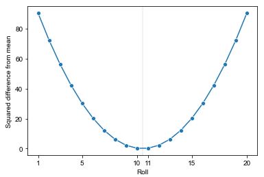
Why squared error?
Why are we calculating average squared difference from the expectation rather than, say, average absolute difference? The answer has to do with the nature of averages. It turns out the average is the \(x\) that minimizes the sum of squared differences,
[\mathrm{sqe}(x, y) = \sum_{n \in 1:N} (y_n - x)^2,]
or equivalently, minimizes the average (or mean) squared difference,
[\mathrm{msqe}(x, y) = \frac{1}{N} \sum_{n \in 1:N} (y_n - x)^2.]
That is,
[\mathrm{avg}(y)
\ =
\frac{1}{N} \sum_{n = 1}^N y_n
\ =
\mathrm{argmin}_x \ \mathrm{msqe}(x, y)]
The notation \(\mathrm{argmin}_x \ f(x)\) is meant to return the \(x\) at which \(f(x)\) takes on its minimum value. For example, \(\mathrm{argmin}_u (u - 1)^2 + 7 = 1\), whereas the minimum value is given by \(\mathrm{min}_u (u - 1)^2 + 7 = 7\).
Averages themselves are important because expectations are defined in terms of averages, and event probabilities are defined in terms of expectations. Furthermore, the central limit theorem governs the convergence of averages as estimates of quantities of interest in terms of squared error.
Standard deviations for scale correction
The difficulty in managing variance is that it has different units than the variable it is measuring the variation of. For example, if \(Y\) represents the fill of a bottle with units in milliliters, then \(\mathrm{var}[Y]\) has units of squared milliliters. Squared milliliters are not natural. As we saw even with the calculation for a single six-sided die, values of 1 and 6 had 6.25 squared difference from the expected value of 3.5, whereas 3 and 4 had only 0.25 squared difference from the expected value. Small values (below one) get smaller (\(0.5^2 = 0.25\)) and large values are amplified (\(2.5^2 = 6.25\)).
Instead of dealing with variance, with its quadratic scale and mismatched units, it is common to convert back at the end to ordinary units by taking a square root. The standard deviation of a random variable is defined as the square root of its variance,
[\mathrm{sd}[Y] = \sqrt{\mathrm{var}\left[ Y \right]}.]
While it is not known why Karl Pearson coined the term “standard deviation”,^[Pearson, K., 1893. Contributions to the mathematical theory of evolution. Philosophical Transactions of the Royal Society of London, Series A. Nov 16: 329–333, which on page 330 coins the term stating only, “standard deviations—a term used in the memoir for what corresponds in frequency curves to the error of mean square.”] the key consideration here is that \(\mathrm{sd}[Y]\) has the same units as the variable \(Y\) itself and is thus much easier to interpret.
Key Points
Joint, Marginal, and Conditional Probabilities
Overview
Teaching: min
Exercises: minQuestions
Objectives
Joint, Marginal, and Conditional Probabilities
Diagnostic accuracy
What if I told you that you just tested positive on a diagnostic test with 95% accuracy, but that there’s only a 16% chance that you have the disease in question? This running example will explain how this can happen.^[The example diagnostic accuracies and disease prevalences we will use for simulation are not unrealistic—this kind of thing happens all the time in practice, which is why there are often batteries of follow-up tests after preliminary positive test results.]
Suppose the random variable \(Z \in 0:1\) represents whether a particular subject has a specific disease.^[\(Z = 1\) if the subject has the disease and \(Z = 0\) if not.] Now suppose there is a diagnostic test for whether a subject has the disease. Further suppose the random variable \(Y \in 0:1\) represents the result of applying the test to the same subject.^[\(Y = 1\) if the test result is positive and \(Y = 0\) if it’s negative.]
Now suppose the test is 95% accurate in the sense that
- if the test is administered to a subject with the disease (i.e., \(Z = 1\)), there’s a 95% chance the test result will be positive (i.e., \(Y = 1\)), and
- if the test is administered to a subject without the disease (i.e., \(Z = 0\)), there’s a 95% chance the test result will be negative (i.e., \(Y = 0)\).
We’re going to pause the example while we introduce the probability notation required to talk about it more precisely. Conditional probability notation expresses the diagnostic test’s accuracy for people have the disease (\(Z = 1\)) as
\(\mbox{Pr}[Y = 1 \mid Z = 1] = 0.95\)\
and for people who don’t have the disease (\(Z = 0\)) as
\(\mbox{Pr}[Y = 0 \mid Z = 0] = 0.95.\)\
We read \(\mbox{Pr}[\mathrm{A} \mid \mathrm{B}]\) as the conditional probability of event \(\mathrm{A}\) given that we know event \(\mathrm{B}\) occurred. Knowing that event \(\mathrm{B}\) occurs often, but not always, gives us information about the probability of \(\mathrm{A}\) occurring.
The conditional probability function \(\mbox{Pr}[\, \cdot \mid \mathrm{B}]\) behaves just like the unconditional probability function \(\mbox{Pr}[\, \cdot \,]\). That is, it satisfies all of the laws of probability we have introduced for event probabilities. The difference is in the semantics—conditional probabilities are restricted to selecting a way the world can be that is consistent with the event \(\mathrm{B}\) occurring.^[Formally, an event \(\mathrm{B}\) is modeled as a set of ways the world can be, i.e., a subset \(\mathrm{B} \subseteq \Omega\) of the sample space \(\Omega\). The conditional probability function \(\mbox{Pr}[\, \cdot \mid \mathrm{B}]\) can be interpreted as an ordinary probability distribution with sample space \(\mathrm{B}\) instead of the original \(\Omega\).]
For example, the sum of exclusive and exhaustive probabilities must be one, and thus the diagnostic error probabilities are one minus the correct diagnosis probabilities,^[These error rates are often called the false positive rate and false negative rate, the positive and negative in this case being the test result and the false coming from not matching the true disease status.]
\(\mbox{Pr}[Y = 0 \mid Z = 1] = 0.05\)\
and
\(\mbox{Pr}[Y = 1 \mid Z = 0] = 0.05.\)\
Conditional probability
Definition: Events A, B are independent if \(P(A\cap B) = P(A)P(B)\)
Note: completely different form disjointness
\(A, B, C\) are independent, if \(P(A, B) = P(A)P(B)\), \(P(A,C) = P(A)P(C)\), \(P(B,C) = P(B)P(C)\) and \(P(A, B, C) = P(A)P(B)P(C)\)
Similarly for events A1,…An
Newton-Pepys Problem(1693)
The Newton–Pepys problem is a probability problem concerning the probability of throwing sixes from a certain number of dice.
In 1693 Samuel Pepys and Isaac Newton corresponded over a problem posed by Pepys in relation to a wager he planned to make. The problem was:
A. Six fair dice are tossed independently and at least one “6” appears.
B. Twelve fair dice are tossed independently and at least two “6”s appear.
C. Eighteen fair dice are tossed independently and at least three “6”s appear.
Solution
Pepys initially thought that outcome C had the highest probability, but Newton correctly concluded that outcome A actually has the highest probability. Quoted from Wikipedia : Newton–Pepys problem
\(P(A) = 1 - (5/6)^6 \approx 0.665\)
\(P(B) = 1 - (5/6)^{12} - 12 *(1/6)(5/6)^{11} \approx 0.619\)
\(P(C) = 1 - \sum_{k=0}^2 \binom{18}{k} (1/6)^k (5/6)^{(18-k)} \approx 0.597\)
Challenge - — How should you update probability/beliefs/uncertainty based on new evidence?
“Conditioning is the soul of statistic”
Conditional Probability
Definition:
\(P(A|B) = \frac{P(A\cap B)} {P(B)}\), if \(P(B) > 0\)
Intuition:
-
Pebble world , there are finite possible outcomes, each one is represented as a pebble. For example, 9 outcomes, that is 9 pebbles , total mass is 1. B: four pebbles, \(P(A|B)\):get rid of pebbles in \(B^c\) , renormalize to make total mass again
-
Frequentist world: repeat experiment many times
(100101101) 001001011 11111111
circle repeatitions where B occurred ; among those , what fraction of time did A also occur?
Theorem
- \(P(A\cap B) = P(B)P(A|B) = P(A)P(B|A)\)\
- \(P(A_1…A_n) = P(A_1)P(A_2|A_1)P(A_3|A_1,A_2)…P(A_n|A_1,A_2…A_{n-1})\)\
- \(P(A|B) = \frac{P(B|A)P(A)}{P(B)}\)\
Thinking conditionally is a condition for thinking
How to solve a problem?
-
Try simple and extreme cases
-
Break up problem into simple pieces
\[P(B) = P(B|A_1)P(A_1) + P(B|A_2)P(A_2) +…P(B|A_n)P(A_n)\]law of total probability
Example 1- Suppose we have 2 random cards from standard deck
Find \(P(both\ aces|have\ ace), P(both\ aces|have\ ace\ of\ spade)\)
Solution
\(P (\text{both aces}|\text{have ace}) = \frac{P(\text{both aces}, \text{have ace})}{P(\text{have ace})} = \frac{\binom{4}{2}/\binom{52}{2}}{1-\binom{48}{2}/\binom{52}{2}} = \frac{1}{33}\)
\(P (both\ aces|have\ ace\ of\ spade) = 3/51 = 1/17\)
Example 2 - Patient get tested for disease afflicts 1% of population, tests positive (has disease)
Suppose the test is advertised as “95% accurate” , suppose this means \(D\): has disease, \(T\): test positive
Solution
Trade-off: It’s rare that the test is wrong, it’s also rare the disease is rare \(\)
\(P(T|D) = 0.95 = P(T^c |D^c)\) \(\)
\(P(D|T) = \frac{P(T|D)P(D)}{P(T)} = \frac{P(T|D)P(D)}{P(T|D)P(D) + P(T|D^c)P(D^c}{}\)
Biohazards
- confusing \(P(A|B)\), \(P(B|A)\) (procecutor’s fallacy)
Ex Sally Clark case, SIDS
want \(P(innocence|evidence)\)
- confusing \(P(A) - prior\) with \(P(A|B)\) - posterior
| [P(A | A) = 1] |
- confusing independent with conditional independent
Definition:
Events \(A,B\) are conditionally independent given \(C\) if \(P(A\cap B|C)\) = \(P(A|C)P(B|C)\)
Does conditional independence given C imply independence ?
Solution
No \(\)
Example - Chess opponent of unknown strength may be that game outcomes are conditionally independent given strength
Does independent imply conditional independent given C?
Solution
No \(\)
Example - A: Fire alarm goes off, cause by : F:fire; C:popcorn. suppose F, C independent But \(\)
\(P(F|A, C^c^) = 1\) not conditionally independent given A
Joint probability
Joint probability notation expresses the probability of multiple events happening. For instance, \(\mbox{Pr}[Y = 1, Z = 1]\) is the probability of both events, \(Y = 1\) and \(Z = 1\), occurring.
In general, if \(\mathrm{A}\) and \(\mathrm{B}\) are events,^[We use capital roman letters for event variables to distinguish them from random variables for which we use capital italic letters.] we write \(\mbox{Pr}[\mathrm{A}, \mathrm{B}]\) for the event of both \(\mathrm{A}\) and \(\mathrm{B}\) occurring. Because joint probability is defined in terms of conjunction (“and” in English), the definition is symmetric, \(\mbox{Pr}[\mathrm{A}, \mathrm{B}] = \mbox{Pr}[\mathrm{B}, \mathrm{A}].\)
In the context of a joint probability \(\mbox{Pr}[\mathrm{A}, \mathrm{B}]\), the single event \(\mbox{Pr}[\mathrm{A}]\) is called a marginal probability.^[Because of symmetry, \(\mbox{Pr}[\mathrm{B}]\) is also a marginal probability.]
Joint probability is defined relative to conditional and marginal probabilities by
[\mbox{Pr}[\mathrm{A}, \mathrm{B}]
\ =
\mbox{Pr}[\mathrm{A} \mid \mathrm{B}] \times \mbox{Pr}[\mathrm{B}].]
In words, the probability of events \(\mathrm{A}\) and \(\mathrm{B}\) occurring is the same as the probability of event \(\mathrm{B}\) occurring times the probability of \(\mathrm{A}\) occurring given that \(\mathrm{B}\) occurs.
The relation between joint and conditional probability involves simple multiplication, which may be rearranged by dividing both sides by \(\mbox{Pr}[\mathrm{B}]\) to yield
[\mbox{Pr}[\mathrm{A} \mid \mathrm{B}]
\ =
\frac{\displaystyle \mbox{Pr}[\mathrm{A}, \mathrm{B}]}
{\displaystyle \mbox{Pr}[\mathrm{B}]}.]
Theoretically, it is simplest to take joint probability as the primitive so that this becomes the definition of conditional probability. In practice, all that matters is the relation between conditional and joint probability.
Dividing by zero: not-a-number or infinity
Conditional probabilities are not well defined in the situation where \(\mbox{Pr}[B] = 0\). In such a situation, \(\mbox{Pr}[\mathrm{A}, \mathrm{B}] = 0\), because \(B\) has probability zero.
In practice, if we try to evaluate such a condition using standard computer floating-point arithmetic, we wind up dividing zero by zero.
Pr_A_and_B = 0.0
Pr_B = 0.0
Pr_A_given_B = Pr_A_and_B / Pr_B
print('Pr[A | B] = ', Pr_A_given_B)
Running that, we get
ZeroDivisionError: float division by zero
The value NaN indicates what is known as the not-a-number
value.^[There are technically two types of not-a-number values in the
IEEE 754 standard, of which we will only consider the non-signaling
version.] This is a special floating-point value that is different
from all other values and used to indicate a domain error on an
operation. Other examples that will return not-a-number values
include log(-1).
If we instead divide a positive or negative number by zero,
print('1.0 / 0.0 = ', 1.0 / 0.0)
print('-3.2 / 0.0 = ', -3.2 / 0.0)
we get
1.0 / 0.0 = Inf
-3.2 / 0.0 = -Inf
These values denote positive infinity (\(\infty\)) and negative infinity (\(-\infty\)), respectively. Like not-a-number, these are special reserved floating-point values with the expected interactions with other numbers.^[For example, adding a finite number and an infinity yields the infinity and subtracting two infinities produces a not-a-number value. For details, see 754-2008—IEEE standard for floating-point arithmetic.]
Simulating the diagnostic example
What we don’t know so far in the running example is what the probability is of a subject having the disease or not. This probability, known as the prevalence of the disease, is often the main quantity of interest in an epidemiological study.
Let’s suppose in our case that 1% of the population has the disease in question. That is, we assume
[\mbox{Pr}[Z = 1] = 0.01]
Now we have enough information to run a simulation of all of the joint probabilities. We just follow the marginal and conditional probabilities. First, we generate \(Z\), whether or not the subject has the disease, then we generate \(Y\), the result of the test, conditional on the disease status \(Z\).
import numpy as np

M = 1000000
z = np.zeros(M)
y = np.zeros(M)

for m in range(M):
    z[m] = np.random.binomial(1, 0.01)
    if z[m] == 1:
        y[m] = np.random.binomial(1, 0.95)
    else:
        y[m] = np.random.binomial(1, 0.05)

print('estimated Pr[Y = 1] = ', np.sum(y) / M)
print('estimated Pr[Z = 1] = ', np.sum(z) / M)
estimated Pr[Y = 1] =  0.058812
estimated Pr[Z = 1] =  0.009844
The program computes the marginals for \(Y\) and \(Z\) directly. This is
straightforward because both \(Y\) and \(Z\) are simulated in every
iteration (as y[m] and z[m] in the code). Marginalization using
simulation requires no work whatsoever.^[Marginalization can be
tedious, impractical, or impossible to carry out analytically.]
Let’s run that with \(M = 100,000\) and see what we get.
import numpy as np

np.random.seed(1234)
M = 100000
z = np.random.binomial(1, 0.01, M)
y = np.where(z == 1, np.random.binomial(1, 0.95, M), np.random.binomial(1, 0.05, M))
print('estimated Pr[Y = 1] = ', np.sum(y) / M)
print('estimated Pr[Z = 1] = ', np.sum(z) / M)
estimated Pr[Y = 1] =  0.05755
estimated Pr[Z = 1] =  0.01008
We know that the marginal \(\mbox{Pr}[Z = 1]\) is 0.01, so the estimate is close to the true value for \(Z\); we’ll see below that it’s also close to the true value of \(\mbox{Pr}[Y = 1]\).
We can also use the simulated values to estimate conditional probabilities. To estimate, we just follow the formula for the conditional distribution,
[\mbox{Pr}[A \mid B]
\ =
\frac{\displaystyle \mbox{Pr}[A, B]}
{\displaystyle \mbox{Pr}[B]}.]
Specifically, we count the number of draws in which both A and B occur, then divide by the number of draws in which the event B occurs.
import numpy as np

np.random.seed(1234)
M = 100000
z = np.random.binomial(1, 0.01, M)
y = np.where(z == 1, np.random.binomial(1, 0.95, M), np.random.binomial(1, 0.05, M))
y1z1 = np.logical_and(y == 1, z == 1)
y1z0 = np.logical_and(y == 1, z == 0)

print('estimated Pr[Y = 1 | Z = 1] = ', np.sum(y1z1) / np.sum(z == 1))
print('estimated Pr[Y = 1 | Z = 0] = ', np.sum(y1z0) / np.sum(z == 0))
We set the indicator variable y1z1[m] to 1 if \(Y = 1\) and \(Z = 1\) in
the \(m\)-th simulation; y1z0 behaves similarly. The operator & is
used for conjuncton (logical and) in the usual way.^[The logical and
operation is often written as && in programming languages to
distinguish it from bitwise and, which is conventionally written &.]
Recall that z == 0
is an array where entry \(m\) is 1 if the condition holds, here \(z^{(m)}
= 0\).
The resulting estimates with \(M = 100,000\) draws are pretty close to the true values,
estimated Pr[Y = 1 | Z = 1] =  0.9454365079365079
estimated Pr[Y = 1 | Z = 0] =  0.048508970421852274
The true values were stipulated as part of the example to be \(\mbox{Pr}[Y = 1 \mid Z = 1] = 0.95\) and \(\mbox{Pr}[Y = 1 \mid Z = 0] = 0.05\). Not surprisingly, knowing the value of \(Z\) (the disease status) provides quite a bit of information about the value of \(Y\) (the diagnostic test result).
Now let’s do the same thing the other way around,and look at the probability of having the disease based on the test result, i.e., \(\mbox{Pr}[Z = 1 \mid Y = 1]\) and \(\mbox{Pr}[Z = 1 \mid Y = 0]\).^[The program is just like the last one.]
print('estimated Pr[Z = 1 | Y = 1] = {:.3f}'.format(sum(y * z) / sum(y)))
print('estimated Pr[Z = 1 | Y = 0] = {:.3f}'.format(sum(z * (1 - y)) / sum(1 - y)))
estimated Pr[Z = 1 | Y = 1] = 0.166
estimated Pr[Z = 1 | Y = 0] = 0.001
Did we make a mistake in coding up our simulation? We estimated \(\mbox{Pr}[Z = 1 \mid Y = 1]\) at around 16%, which says that if the subject has a positive test result (\(Y = 1\)), there is only a 16% chance they have the disease (\(Z = 1\)). How can that be when the test is 95% accurate and simulated as such?
The answer hinges on the prevalence of the disease. We assumed only 1% of the population suffered from the disease, so that 99% of the people being tested were disease free. Among the disease free (\(Z = 0\)) that are tested, 5% of them have false positives (\(Y = 1\)). That’s a lot of patients, around 5% times 99%, which is nearly 5% of the population. On the other hand, among the 1% of the population with the disease, almost all of them test positive. This means roughly five times as many disease-free subjects test positive for the disease as disease-carrying subjects test positive.
Analyzing the diagnostic example
The same thing can be done with algebra as we did in the previous section with simulations.^[Computationally, precomputed algebra is a big win over simulations in terms of both compute time and accuracy. It may not be a win when the derivations get tricky and human time is taken into consideration.] Now we can evaluate joint probabilities, e.g.,
[\begin{array}{rcl}
\mbox{Pr}[Y = 1, Z = 1]
& = & \mbox{Pr}[Y = 1 \mid Z = 1] \times \mbox{Pr}[Z = 1]
\[4pt]
& = & 0.95 \times 0.01
& = & 0.0095.
\end{array}]
Similarly, we can work out the probability the remaining probabilities in the same way, for example, the probability of a subject having the disease and getting a negative test result,
[\begin{array}{rcl}
\mbox{Pr}[Y = 0, Z = 1]
& = & \mbox{Pr}[Y = 0 \mid Z = 1] \times \mbox{Pr}[Z = 1]
\[4pt]
& = & 0.05 \times 0.01
& = & 0.0005.
\end{array}]
Doing the same thing for the disease-free patients completes a four-by-four table of probabilities,
[\begin{array}{|r|r|r|} \hline \mbox{Probability} & Y = 1 & Y = 0 \ \hline Z = 1 & 0.0095 & 0.0005 \ \hline Z = 0 & 0.0450 & 0.8500 \ \hline \end{array}]
For example, the top-left entry records the fact that \(\mbox{Pr}[Y = 1, Z = 1] = 0.0095.\) The next entry to the right indicates that \(\mbox{Pr}[Y = 0, Z = 1] = 0.0005.\)
The marginal probabilities (e.g., \(\mbox{Pr}[Y = 1]\)) can be computed by summing the probabilities of all alternatives that lead to \(Y = 1\), here \(Z = 1\) and \(Z = 0\)
[\mbox{Pr}[Y = 1]
\ =
\mbox{Pr}[Y = 1, Z = 1]
- \mbox{Pr}[Y = 1, Z = 0]]
We can extend our two-by-two table by writing the sums in what would’ve been the margins of the original table above.
[\begin{array}{|r|r|r|r|} \hline \mbox{Probability} & Y = 1 & Y = 0 & Y = 1 \ \mbox{or} \ Y = 0 \ \hline Z = 1 & 0.0095 & 0.0005 & \mathit{0.0100} \ \hline Z = 0 & 0.0450 & 0.8500 & \mathit{0.9900} \ \hline Z = 1 \ \mbox{or} \ Z = 0 & \mathit{0.0545} & \mathit{0.8505} & \mathbf{1.0000} \ \hline \end{array}]
Here’s the same table with the symbolic values.
[\begin{array}{|r|r|r|r|} \hline \mbox{Probability} & Y = 1 & Y = 0 & Y = 1 \ \mbox{or} \ Y = 0 \ \hline Z = 1 & \mbox{Pr}[Y = 1, Z = 1] & \mbox{Pr}[Y = 0, Z = 1] & \mbox{Pr}[Z = 1] \ \hline Z = 0 & \mbox{Pr}[Y = 1, Z = 0] & \mbox{Pr}[Y = 0, Z = 0] & \mbox{Pr}[Z = 0] \ \hline Z = 1 \ \mbox{or} \ Z = 0 & \mbox{Pr}[Y = 1] & \mbox{Pr}[Y = 0] & \mbox{Pr}[ \ ] \ \hline \end{array}]
For example, that \(\mbox{Pr}[Z = 1] = 0.01\) can be read off the top of the right margin column—it is the sum of the two table entries in the top row, \(\mbox{Pr}[Y = 1, Z = 1]\) and \(\mbox{Pr}[Y = 0, Z = 1]\).
In the same way, \(\mbox{Pr}[Y = 0] = 0.8505\) can be read off the right of the bottom margin row, being the sum of the entries in the right column, \(\mbox{Pr}[Y = 0, Z = 1]\) and \(\mbox{Pr}[Y = 0, Z = 0]\).
The extra headings define the table so that each entry is the probability of the event on the top row and on the left column. This is why it makes sense to record the grand sum of 1.00 in the bottom right of the table.
Joint and conditional distribution notation
Recall that the probability mass function \(p_Y(y)\) for a discrete random variable \(Y\) is defined by
[p_Y(y) = \mbox{Pr}[Y = y].]
As before, capital \(Y\) is the random variable, \(y\) is a potential value for \(Y\), and \(Y = y\) is the event that the random variable \(Y\) takes on value \(y\).
The joint probability mass function for two discrete random variables \(Y\) and \(Z\) is defined by the joint probability,
[p_{Y,Z}(y, z) = \mbox{Pr}[Y = y, Z = z].]
The notation follows the previous notation with \(Y, Z\) indicating that the first argument is the value of \(Y\) and the second that of \(Z\).
Similarly, the conditional probablity mass function is defined by
[p_{Y \mid Z}(y \mid z) = \mbox{Pr}[Y = y \mid Z = z].]
It can equivalently be defined as
[p_{Y \mid Z}(y \mid z)
\ =
\frac{\displaystyle p_{Y, Z}(y, z)}
{\displaystyle p_{Z}(z)}.]
The notation again follows that of the conditional probability function through which the conditional probability mass function is defined.
Bayes’s Rule
Bayes’s rule relates the conditional probability \(\mbox{Pr}[\mathrm{A} \mid \mathrm{B}]\) for events \(\mathrm{A}\) and \(\mathrm{B}\) to the inverse conditional probability \(\mbox{Pr}[\mathrm{A} \mid \mathrm{B}]\) and the marginal probability \(\mbox{Pr}[\mathrm{B}]\). The rule requires a partition of the event \(\mathrm{A}\) into events \(\mathrm{A}_1, \ldots, \mathrm{A}_K\), which are mutually exclusive and exhaust \(\mathrm{A}\). That is,
[\mbox{Pr}[\mathrm{A}k, \mathrm{A}{k’}] = 0 \ \ \mbox{if} \ \ k \neq k’,]
and
[\begin{array}{rcl} \mbox{Pr}[\mathrm{A}] & = & \mbox{Pr}[\mathrm{A}1] + \cdots + \mbox{Pr}[\mathrm{A}_K]. \[3pt] & = & \sum{k \in 1:K} \mbox{Pr}[\mathrm{A}_k]. \end{array}]
The basic rule of probability used to derive each line is noted to the right.
[\begin{array}{rcll} \mbox{Pr}[\mathrm{A} \mid \mathrm{B}] & = & \frac{\displaystyle \mbox{Pr}[\mathrm{A}, \mathrm{B}]} {\displaystyle \mbox{Pr}[\mathrm{B}]} & \ \ \ \ \mbox{[conditional definition]} \[6pt] & = & \frac{\displaystyle \mbox{Pr}[\mathrm{B} \mid \mathrm{A}] \times \mbox{Pr}[\mathrm{A}]} {\displaystyle \mbox{Pr}[\mathrm{B}]} & \ \ \ \ \mbox{[joint definition]} \[6pt] & = & \frac{\displaystyle \mbox{Pr}[\mathrm{B} \mid \mathrm{A}] \times \mbox{Pr}[\mathrm{A}]} {\displaystyle \sum_{k \in 1:K} \displaystyle \mbox{Pr}[\mathrm{B}, \mathrm{A}k]} & \ \ \ \ \mbox{[marginalization]} \[6pt] & = & \frac{\displaystyle \mbox{Pr}[\mathrm{B} \mid \mathrm{A}] \times \mbox{Pr}[\mathrm{A}]} {\displaystyle \sum{k \in 1:K} \mbox{Pr}[\mathrm{B} \mid \mathrm{A}_k] \times \mbox{Pr}[\mathrm{A}_k]}. & \ \ \ \ \mbox{[joint definition]} \end{array}]
Letting \(\mathrm{A}\) be the event \(Y = y\), \(\mathrm{B}\) be the event \(Z = z\), and \(A_k\) be the event \(Y = k\), Bayes’s rule can be instantiated to
[\mbox{Pr}[Y = y \mid Z = z]
\ =
\frac{\displaystyle
\mbox{Pr}[Z = z \mid Y = y] \times \mbox{Pr}[Y = y]}
{\displaystyle
\sum_{y’ \in 1:K} \mbox{Pr}[Z = z \mid Y = y’] \times \mbox{Pr}[Y = y’]}.]
This allows us to express Bayes’s rule in terms of probability mass functions as
[p_{Y \mid Z}(y \mid z)
\ =
\frac{\displaystyle p_{Z \mid Y}(z \mid y) \times p_{Y}(y)}
{\displaystyle \sum_{y’ \in 1:K} p_{Z \mid Y}(z \mid y’) \times p_Y(y’)}.]
Bayes’s rule can be extended to infinite partitions of the event \(B\), or in the probability mass function case, a variable \(Y\) taking on infinitely many possible values.
Fermat and the problem of points
Blaise Pascal and Pierre de Fermat studied the problem of how to divide the pot^[The pot is the total amount bet by both players.] of a game of chance that was interrupted before it was finished. As a simple example, Pascal and Fermat considered a game in which each turn a fair coin was flipped, and the first player would score a win a point if the result was heads and the second player if the result was tails. The first player to score ten points wins the game.
Now suppose a game is interrupted after 15 flips, at a point where the first player has 8 points and the second player only 7. What is the probability of the first player winning the match were it to continue?
We can put that into probability notation by letting \(Y_n\) be the number of points for the first player after \(n\) turns.
\(Y_{n, 1}\) be the number of heads for player 1 after \(n\) flips, \(Y_{n, 2}\) be the same for player 2. Let \(Z\) be a binary random variable taking value 1 if the first player wins and 0 if the other player wins. Fermat managed to evaluate a formula like Fermat evaluated \(\mbox{Pr}[Z = 1 \mid Y_{n, 1} = 8, Y_{n, 2} = 7]\) by enumerating the possible game continuations and adding up the probabilities of the ones in which the first player wins.
We can solve Fermat and Pascal’s problem by simulation. As usual, our
estimate is just the proportion of the simulations in which the first
player wins. The value of pts must be given as input—that is the
starting point for simulating the completion of the game, assuming
neither player yet has ten points.^[For illustrative purposes only!
In robust code, validation should produce diagnostic error messages
for invalid inputs.]
import numpy as np

np.random.seed(1234)
M = 100000
win = np.zeros(M)
for m in range(M):
    pts = [0, 0]
    while pts[0] < 10 and pts[1] < 10:
        toss = np.random.uniform()
        if toss < 0.5:
            pts[0] += 1
        else:
            pts[1] += 1
    if pts[0] == 10:
        win[m] = 1
    else:
        win[m] = 0

print('est. Pr[player 1 wins] =', np.mean(win))
est. Pr[player 1 wins] = 0.50181
If the while-loop terminates because one player has ten points, then
wins[m] must have been set in the previous value of the loop.^[In
general, programs should be double-checked (ideally by a third party)
to make sure invariants like this one (i.e., win[m] is always set)
actually hold. Test code goes a long way to ensuring robustness.]
Let’s run that a few times with \(M = 100,000\), starting with the
pts set to (8, 7), to simulate Fermat and Pascal’s problem.
import numpy as np

np.random.seed(1234)

for k in range(1, 6):
    M = 100000
    game_wins = 0

    for m in range(M):
        wins = [8, 7]

        while wins[0] < 10 and wins[1] < 10:
            toss = np.random.binomial(1, 0.5)
            winner = 1 if toss == 1 else 2
            wins[winner - 1] += 1

            if wins[0] == 10:
                game_wins += 1

    print(f'est. Pr[player 1 wins] = {game_wins / M:.3f}')
est. Pr[player 1 wins] = 0.686
est. Pr[player 1 wins] = 0.687
est. Pr[player 1 wins] = 0.688
est. Pr[player 1 wins] = 0.687
est. Pr[player 1 wins] = 0.686
This is very much in line with the result Fermat derived by brute force, namely \(\frac{11}{16} \approx 0.688.\)^[There are at most four more turns required, which have a total of \(2^4 = 16\) possible outcomes, HHHH, HHHT, HHTH, \(\ldots,\) TTTH, TTTT, of which 11 produce wins for the first player.]
Independence of random variables
Informally, we say that a pair of random variables is independent if knowing about one variable does not provide any information about the other. If \(X\) and \(Y\) are the variables in question, this property can be stated directly in terms of their probability mass functions as
| [p_{X}(x) = p_{X | Y}(x \mid y).] |
In practice, we use an equivalent definition. Random variables \(X\) and \(Y\) are said to be independent if
[p_{X,Y}(x, y) = p_X(x) \times p_Y(y).]
for all \(x\) and \(y\).^[This is equivalent to requiring the events \(X \leq x\) and \(Y \leq y\) to be independent for every \(x\) and \(y\). Events A and B are said to be independent if \(\mbox{Pr}[\mathrm{A}, \mathrm{B}] \ = \ \mbox{Pr}[\mathrm{A}] \times \mbox{Pr}[\mathrm{B}]\).]
By way of example, we have been assuming that a fair dice throw involves the throw of two independent and fair dice. That is, if \(Y_1\) is the first die and \(Y_2\) is the second die, then \(Y_1\) is independent of \(Y_2\).
In the diagnostic testing example, the disease state \(Z\) and the test result \(Y\) are not independent.^[That would be a very poor test, indeed!]. This can easily be verified because \(p_{Y|Z}(y \mid z) \neq p_Y(y)\).
Independence of multiple random variables
It would be nice to be able to say that a set of random \(Y_1, \ldots, Y_N\) was independent if each of its pairs of random variables was independent. We’d settle for being able to say that the joint probability factors into the product of marginals,
[p_{Y_1, \ldots, Y_N}(y_1, \ldots, y_N)
\ =
p_{Y_1}(y1) \times \cdots \times p_{Y_N}(y_N).]
But neither of these is enough.^[Analysis in general and probability theory in particular defeat simple definitions with nefarious edge cases.] For a set of random variables to be independent, the probability of each of its subsets must factor into the product of its marginals.^[More precisely, \(Y_1, \ldots, Y_N\) are independent if for every \(M \leq N\) and permutation \(\pi\) of \(1:N\) (i.e., a bijection between \(1:N\) and itself), we have \(\begin{array}{l} \displaystyle p_{Y_{\pi(1)}, \ldots, Y_{\pi(M)}}(u_1, \ldots, u_M) \\ \displaystyle \mbox{ } \ \ \ = \ p_{Y_{\pi(1)}}(u_1) \times \cdots \times p_{Y_{\pi(M)}}(u_M) \end{array}\) for all \(u_1, \ldots, u_M.\)]
Conditional independence
Often, a pair of variables are not independent only because they both depend on a third variable. The random variables \(Y_1\) and \(Y_2\) are said to be conditionally independent given the variable \(Z\) if they are independent after conditioning,
[p_{Y_1, Y_2 \mid Z}(y_1, y_2 \mid z)
\ =
p_{Y_1 \mid Z}(y_1 \mid z) \times p_{Y_2 \mid Z}(y_2 \mid z).]
Conditional expectations
The expectation \(\mathbb{E}[Y]\) of a random variable \(Y\) is its average value (weighted by density or mass, depending on whether it is continuous or discrete). The conditional expectation \(\mathbb{E}[Y \mid A]\) given some event \(A\) is defined to be the average value of \(Y\) conditioned on the event \(A\),
[\mathbb{E}[Y \mid A]
\ =
\int_Y y \times p_{Y \mid A}(y \mid A) \, \mathrm{d} y,]
where \(p_{Y \mid A}\) is the density of \(Y\) conditioned on event \(A\) occurring. This conditional density \(p_{Y \mid A}\) is defined just like the ordinary density \(p_Y\) only with the conditional cumulative distribution function \(F_{Y \mid A}\) instead of the standard cumulative distribution function \(F_Y\),
[p_{Y \mid A}(y \mid A)
\ =
\frac{\mathrm{d}}{\mathrm{d} y} F_{Y \mid A}(y \mid A).]
The conditional cumulative distribution function \(F_{Y \mid A}\) is, in turn, defined by the conditioning on the event probability,
[F_{Y \mid A}(y \mid A)
\ =
\mbox{Pr}[Y < y \mid A].]
This also works to condition on zero probability events, such as \(\Theta = \theta\), by taking the usual definition of conditional density,
[\mathbb{E}[Y \mid \Theta = \theta]
\ =
\int_Y y \times p_{Y \mid \Theta}(y \mid \theta) \, \mathrm{d}y.]
When using discrete variables, integrals are replaced with sums.
Independent and identically distributed variables
If the variables \(Y_1, \ldots, Y_N\) are not only independent, but also have the same probability mass functions (i.e., \(p_{Y_n} = p_{Y_{m}}\) for all \(m, n \in 1:N\)), we say that they are independent and identically distributed, or “iid” for short. Many of our statistical models, such as linear regression, will make the assumption that observations are conditionally independent and identically distributed.
Key Points
Finite-State Markov Chains
Overview
Teaching: min
Exercises: minQuestions
Objectives
Finite-State Markov Chains
Random processes
A finite sequence of random variables is said to be a random vector. An infinite sequence
[Y = Y_1, Y_2, \ldots]
of random variables is said to be a random process.^[We consider only discrete random processes where the set of indexes is the counting numbers \(1, 2, 3, \ldots\). Nevertheless, the set of indexes is infinite, so much of the approach to finite vectors has to be reworked.] A trivial example is a sequence of independent Bernoulli trials in which each \(Y_t\) is drawn independently according to \(Y_t \sim \mbox{bernoulli}(\theta)\). A sequence of independent Bernoulli trials is called a Bernoulli process.
In this chapter, we will restrict attention to processes \(Y\) whose elements take on values \(Y_t \in 0:N\) or \(Y_t \in 1:N\) for some fixed \(N\).^[The choice of starting at 0 or 1 is a convention that varies by distribution. For example, Bernoulli and binomial variates may take on value zero, but categorical values take on values in \(1:N\).] The Bernoulli process is finite in this sense because each \(Y_t\) takes on boolean values, so that \(Y_t \in 0:1\).
Finite-State Markov chains
A random process \(Y\) is said to be a Markov chain if each element is generated conditioned on only the previous element, so that
[p_{Y_{t + 1} \mid Y_1, \ldots, Y_t}(y_{t + 1} \mid y_1, \ldots, y_t)
\ =
p_{Y_{t + 1} \mid Y_t}(y_{t + 1} \mid y_t)]
holds for all \(y_1, \ldots, y_{t + 1}\). In this chapter, we only consider Markov chains in which the \(Y_t\) are finite random variables taking on values \(Y_t \in 0:N\) or \(Y_t \in 1:N\), the range depending on the type of variable.^[We generalize in two later chapters, first to Markov chains taking on countably infinite values and then to ones with continuous values.]
The Bernoulli process discussed in the previous section is a trivial example of a finite Markov chain. Each value is generated independently, so that for all \(y_1, \ldots, y_{t+1}\), we have
[\begin{array}{rcl} p_{Y_{t+1} \mid Y_1, \ldots, Y_t}(y_{t+1} \mid y_1, \ldots, y_t) & = & p_{Y_{t+1} \mid Y_t}(y_{t+1} \mid y_t) \[4pt] = \mbox{bernoulli}(y_{t+1} \mid \theta). \end{array}]
Fish in the stream
Suppose a person is ice fishing for perch and pike, and notes that if they catch a perch, it is 95% likely that the next fish they catch is a perch, whereas if they catch a pike, it is 20% likely the next fish they catch is a pike.^[This is a thinly reskinned version of the classic exercise involving cars and trucks from Ross, S.M.,2014. Introduction to Probability Models. Tenth edition. Academic Press. Exercise 30, page 279.] We’ll treat the sequence of fish types as a random process \(Y = Y_1, Y_2, \ldots\) with values
[Y_t=]
[\begin{cases} 1 & \mbox{if fish t is a pike, and} \[4pt] 2 & \mbox{if fish t is a perch.} \end{cases}]
The sequence \(Y\) forms a Markov chain with transition probabilities
[\begin{array}{rcl} \mbox{Pr}[Y_{t + 1} = 1 \mid Y_t = 1] & = & 0.20 \[4pt] \mbox{Pr}[Y_{t + 1} = 1 \mid Y_t = 2] & = & 0.05 \end{array}]
The easiest way to visual a Markov chain with only a few states is as a state transition diagram. In the case of the pike and perch, the transition diagram is as follows.
State diagram for finite Markov chain generating sequences of fishes. The last fish observed determines the current state and the arrows indicate transition probabilities to the next fish observed.
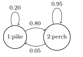 Like all such transition graphs, the probabilities on the edges going
out of a node must sum to one.
Like all such transition graphs, the probabilities on the edges going
out of a node must sum to one.
Let’s simulate some fishing. The approach is to generate the type of each fish in the sequence, then report the overall proportion of pike.^[With some sleight of hand here for compatibility with Bernoulli variates and to facilitate computing proportions, we have recoded perch as having value 0 rather than 2.] We will start with a random fish drawn according to \(\mbox{bernoulli(1/2)}\).
import numpy as np

T = 100 # number of time points
y = np.zeros(T, dtype=int) # initialize array of outcomes
y[0] = np.random.binomial(1, 0.5) # generate first outcome

for t in range(1, T):
    p = 0.2 if y[t-1] == 1 else 0.05 # determine success probability
    y[t] = np.random.binomial(1, p) # generate outcome

prop = np.mean(y) # calculate proportion of 1's
print(f"Simulated proportion of 1's: {prop:.2f}")
Simulated proportion of 1's: 0.08
Now let’s assume the fish are really running, and run a few simulated chains until \(T = 10,000\).
import numpy as np

np.random.seed(1234)
T = 10000
M = 5
for k in range(M):
    y = np.zeros(T, dtype=int)
    y[0] = np.random.binomial(1, 0.5)
    for t in range(1, T):
        p = 0.2 if y[t-1] == 1 else 0.05
        y[t] = np.random.binomial(1, p)
    prop = np.mean(y)
    print(f"Simulated proportion of 1's: {prop:.3f}")
Simulated proportion of 1's: 0.058
Simulated proportion of 1's: 0.063
Simulated proportion of 1's: 0.060
Simulated proportion of 1's: 0.058
Simulated proportion of 1's: 0.060
The proportion of pike is roughly 0.06.
Ehrenfest’s Urns
Suppose we have two urns, with a total of \(N\) balls distributed between them. At each time step, a ball is chosen uniformly at random from among the balls in both urns and moved to the other urn.^[This model was originally introduced as an example of entropy and equilibrium in P. Ehrenfest and T. Ehrenfest. 1906. Über eine Aufgabe aus der Wahrscheinlichkeitsrechnung, die mit der kinetischen Deutung der Entropievermehrung zusammenhängt. Mathematisch-Naturwissenschaftliche Blätter No. 11 and 12.]
The process defines a Markov chain \(Y\) where transitions are governed by
\(p_{Y_{t+1} \mid Y_t}(y_{t+1} \mid y_t)\) \(= \begin{cases} \displaystyle \frac{y_t}{N} & \mbox{if } \ y_{t + 1} = y_t - 1, \ \mbox{and} \\[6pt] \displaystyle 1 - \frac{y_t}{N} & \mbox{if } \ y_{t + 1} = y_t + 1. \end{cases}\)
The transition probabilities make sure that the value of \(Y_t\) remains between 0 and \(N\). For example,
[\mbox{Pr}[Y_{t + 1} = 1 \mid Y_t = 0] = 1]
because \(1 - \frac{y_t}{N} = 1\). Similarly, if \(Y_t = N\), then \(Y_{t+1} = N - 1\).
What happens to the distribution of \(Y_t\) long term? It’s easy to
compute by simulation of a single long chain:^[We’ve used a function
borrowed from R here called table, defined by \(\mbox{table}(y, A,
B)[n] = \sum_{t=1}^T \mbox{I}[y_t = n]\) for \(n \in A:B\). For example, if \(y =
(0, 1, 2, 1, 1, 3, 2, 2, 1),\) then \(\mbox{table}(y, 0, 4) = (1, 4,
3, 1, 0),\) because there is one 0, four 1s, three 2s, a single 3, and
no 4s among the values of \(y\).]
import numpy as np

N = 100 # population size
T = 1000 # number of time points
y = np.zeros(T, dtype=int) # initialize array of counts
z = np.zeros(T, dtype=int) # initialize array of outcomes
y[0] = N // 2 # set initial count to N/2

for t in range(1, T):
    z[t] = np.random.binomial(1, y[t-1]/N) # generate outcome
    y[t] = y[t-1] - 1 if z[t] else y[t-1] + 1 # update count

p_Y_t_hat = np.bincount(y, minlength=N+1) / T # calculate proportion of counts
Let’s run that with \(N = 10\) and \(T = 100,000\) and display the results as a bar plot.
Long-term distribution of number of balls in the first urn of the Ehrenfest model in which \(N\) balls are distributed between two urns, then at each time step, a ball is chosen uniformly at random move to the other urn. The simulation is based on total of \(T = 100,000\) steps with \(N = 10\) balls, starting with 5 balls in the first urn. The points on the top of the bars are positioned at the mass defined by the binomial distribution, \(\\mbox{binomial}(Y_t \\mid 10, 0.5)\).
import numpy as np
import pandas as pd
import matplotlib.pyplot as plt
from scipy.stats import binom
from plotnine import *

np.random.seed(1234)
N = 10
T = 100000
y = np.zeros(T)
y[0] = 5

for t in range(1, T):
    z_t = np.random.binomial(1, y[t-1]/N)
    y[t] = y[t-1] - z_t + (1 - z_t)

ehrenfest_df = pd.DataFrame({'x': np.arange(1, T+1), 'y': y})

ehrenfest_plot = (
    ggplot(data=ehrenfest_df, mapping=aes(x='y')) +
    geom_bar(color='black', fill='#ffffe8', size=0.2) +
    geom_point(data=pd.DataFrame({'x': np.arange(11), 'y': T * binom.pmf(np.arange(11), 10, 0.5)}),
               mapping=aes(x='x', y='y'), size=3, alpha=0.5) +
    scale_x_continuous(breaks=[0, 2, 4, 6, 8, 10]) +
    scale_y_continuous(breaks=np.arange(0, 300000, 50000), labels=[str(x) for x in np.arange(0, 0.6, 0.1)]) +
    xlab('Y[t]') +
    ylab('proportion')
)

print(ehrenfest_plot)
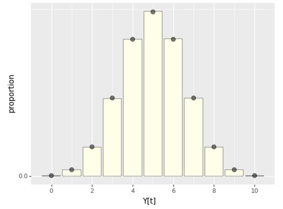
The distribution of \(Y_t\) values is the binomial distribution, as shown by the agreement between the points (the binomial probability mass function) and the bars (the empirical proportion \(Y_t\) spent in each state).^[In the Markov chain Monte Carlo chapter later in the book, we will see how to construct a Markov chain whose long-term frequency distribution matches any given target distribution.]
Page Rank and the random surfer
Pagerank,^[Page, L., Brin, S., Motwani, R. and Winograd, T., 1999. The PageRank citation ranking: Bringing order to the web. Stanford InfoLab Technical Report. Section 2.5 Random Surfer Model.] the innovation behind the original Google search engine ranking system, can be modeled in terms of a random web surfer whose behavior determines a Markov chain. The web is modeled as a set of pages, each of which has a set of outgoing links to other pages. When viewing a particular page, our random surfer chooses the next page to visit by
-
if the current page has outgoing links, then with probability \(\lambda\), choose the next page uniformly at random among the outgoing links,
-
otherwise (with probability \(1 - \lambda\)), choose the next page to visit uniformly at random among all web pages.
Translating this into the language of random variables, let \(Y = Y_1, Y_2, \ldots\) be the sequence of web pages visited. Our goal now is to define the transition function probabilistically so that we may simulate the random surfer. Let \(L_i \subseteq 1:N\) be the set of outgoing links from page \(i\); each page may have any number of outgoing links from \(0\) to \(N\).
The process \(Y\) is most easily described in terms of an auxiliary process \(Z = Z_1, Z_2, \ldots\) where \(Z_t\) represents
the decision whether to jump to a link from the current page. We define \(Z\) by setting \(Z_t = 0\) if the page \(Y_t\) has no outgoing links, and otherwise setting
[Z_t \sim \mbox{bernoulli}(\lambda).]
If \(Z_t = 1\), we can generate \(Y_{t+1}\) uniformly from the links \(L_{Y_t}\) from page \(Y_t\),
[Y_{t + 1} \sim \mbox{uniform}\left( L_{Y_t} \right).]
If \(Z_t = 0\), we simply choose a web page uniformly at random from among all \(N\) pages,
[Y_{t+1} \sim \mbox{uniform}(1:N).]
This sequence is easy to simulate with L[n] denoting the outgoing
links from page n. We start from a page y[1] chosen uniformly at
random among all the pages. Then we just simulate subsequent pages
according to the process described above.
import numpy as np

# Define L and lambda
L = {1: [2, 3, 4], 2: [4], 3: [4], 4: []}
lam = 0.85

# Set initial values
N = 4
T = 10
y = np.zeros(T, dtype=int)
z = np.zeros(T, dtype=int)

# Set initial value for y
y[0] = np.random.randint(1, N+1)

# Simulate y and z
for t in range(1, T):
    last_page = y[t - 1]
    out_links = L[last_page]
    z[t] = 0 if not out_links else np.random.binomial(1, lam)
    y[t] = np.random.choice(out_links) if z[t] else np.random.randint(1, N+1)

print(y)
[4 1 4 2 4 1 4 1 2 4]
Suppose we have the following graph. A simplified web. Each node represents a web page and each edge is a directed link from one page to another web page.
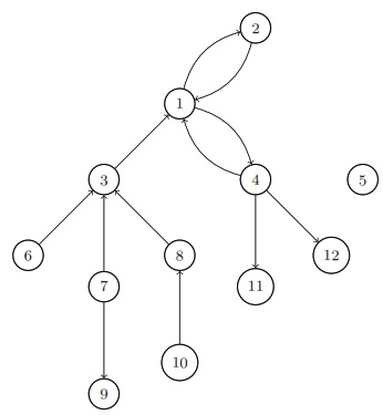
We can simulate \(T = 100,000\) page visits using the algorithm shown above and display the proportion of time spent on each page.
Proportion of time spent on each page by a random surfer taking \(T = 100,000\) page views starting from a random page with a web structured as in the previous diagram.
import numpy as np
import pandas as pd
import matplotlib.pyplot as plt
import seaborn as sns
from scipy.stats import bernoulli

L = np.zeros((12, 12))
L[[0, 2], [1, 3]] = 1
L[1, 0] = 1
L[2, 0] = 1
L[[3, 10, 11], [0, 9, 10]] = 1
L[4, :] = 1
L[5, 2] = 1
L[[6, 8], [2, 8]] = 1
L[7, 2] = 1
L[8, :] = 1
L[9, 7] = 1
L[10, :] = 1
L[11, :] = 1

lmbda = 0.90
theta = np.zeros((12, 12))
for i in range(12):
    if np.sum(L[i, :]) == 0:
        theta[i, :] = np.repeat(1/12, 12)
    else:
        theta[i, :] = lmbda * L[i, :] / np.sum(L[i, :]) + \
                      (1 - lmbda) * np.repeat(1/12, 12)

np.random.seed(1234)
T = int(1e5)
y = np.zeros(T, dtype=int)
y[0] = np.random.choice(12, 1)[0]
for t in range(1, T):
    y[t] = np.random.choice(12, 1, p=theta[y[t-1], :])[0]

visited = np.bincount(y)

pagerank_df = pd.DataFrame({'x': range(1, T+1), 'y': y})

pagerank_plot = (sns
                 .catplot(x='y', data=pagerank_df, kind='count', color='#ffffe8', edgecolor='black', linewidth=0.2)
                 .set(xlabel='page', ylabel='rank (proportion of time on page)',
                      xticks=np.arange(12), yticks=[0, 0.1*T, 0.2*T, 0.3*T], yticklabels=[0, 0.1, 0.2, 0.3])
                 .fig
                )
sns.despine()
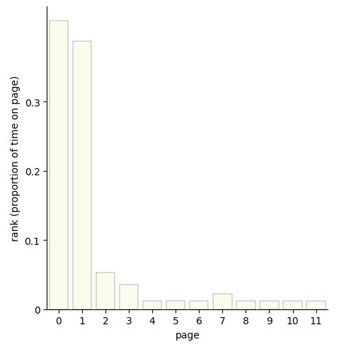
Page 1 is the most central hub. Pages 5, 6, 7, and 10 have no links coming into them and can only be visited by random chance, so all should have the same chance of being visited by the random surfer. Pages 11 and 12 are symmetric, and indeed have the same probability. There is a slight difference between the views of page 9 and 10 in that it possible to get to 9 from 7, but 10 is only visited by chance.
For a Markox transition matrix, the limiting probabilities of being in a certain state as \(n \rightarrow \infty\) are given by the solution to the following set of linear equations. \(p_j^* = \sum_{i=1}^{\infty} p_i^* p_{ij}\)
1. A number from \(1\) to \(m\) is chosen at random, at each of the times \(t = 1, 2, . . .\). A system is said to be in the state \(e_{0}\), if no number has yet been chosen, and in the state \(e_{i}\), if the largest number so far chosen is \(i\). Show that the random process described by this model is a Markov chain. Find the corresponding transition probabilities \(p_{ij} (i, j= 0, 1 , . . . , m)\).
Solution
Since state \(i\) signifies that the highest number chosen so far is \(i\),
what is the probability the next number is lower than \(i\) and you stay in state \(i\)? Well, there are \(m\) possible numbers that could get picked and \(i\) of them are less than or equal to \(i\) giving:
\(p_{ii} = \frac{i}{m}\)
What now if we’re in \(i\) and we want to know what the probability of being in state \(j\) is next.
Well, if \(j<i\) then it’s zero because you can’t go to a lower number in this game.
If, however, \(j\) is not lower then there are \(m\) possible numbers that could get called and only one of them is \(j\), giving:
\(p_{ij} = \frac{1}{m}, j>i\)
\(p_{ij} = 0, j<i\)
Solution
To show that the random process described by this model is a Markov chain, we need to demonstrate that the future state of the process depends only on the current state and not on any of the past states. In this case, the current state is determined by the largest number chosen so far, and the future state is determined by the next number that is chosen.
Formally, we can say that the Markov property holds if:
\(P\left(X_{t+1}=j|X_{t}=i,X_{t-1}=i_{t-1},...,X_{1}=i_{1}\right)= P\left(X_{t+1}=j∣X_{t}=i\right)\)
where \(X_t\) denotes the state of the system at time \(t\), and \(P(X_{t+1}=j | X_t=i)\) represents the probability of transitioning from state \(i\) to state \(j\).
In this case, since the future state depends only on the largest number chosen so far (i.e., the current state) and the next number that is chosen, we can say that the Markov property holds.
The transition probabilities can be calculated as follows:
Let \(p_i\) be the probability that the largest number chosen so far is \(i\).
Then, at any given time \(t\), the probability of choosing a number greater than \(i\) is \((m-i)/m\), and the probability of choosing a number less than or equal to \(i\) is \(i/m\).
Therefore, we can write the transition probabilities as:
\(p_{e_0,e_1} = \frac{1}{m}\)
\(p_{e_i,e_{i+1}} = \frac{m-i}{m}\), for \(i = 0,1,...,m-1\)
\(p_{e_i,e_j} = \frac{i}{m}\), for \(j \le i, i = 1,...,m\)
\(p_{e_i,e_0}= 1 - p_{e_i,e_{i+1}} - \sum_{j=1}^{i}p_{e_i,e_j}\), where the sum is taken over all \(j \le i, i = 1,...,m\)
Note that \(p_{e_i,e_0}\) represents the probability of starting over (i.e., going back to the state \(e_0\)) after reaching state \(e_i\).
These transition probabilities satisfy the Markov property, and therefore, the random process described by this model is a Markov chain.
2. In the preceding problem, which states are persistent and which transient?
Solution
Since state \(i\) signifies that the highest number chosen so far is \(i\),
what is the probability the next number is lower than \(i\) and you stay in state \(i\)? Well, there are \(m\) possible numbers that could get picked and \(i\) of them are less than or equal to \(i\) giving:
\(p_{ii} = \frac{i}{m}\)
What now if we’re in \(i\) and we want to know what the probability of being in state \(j\) is next.
Well, if \(j<i\) then it’s zero because you can’t go to a lower number in this game.
If, however, \(j\) is not lower then there are \(m\) possible numbers that could get called and only one of them is \(j\), giving:
\(p_{ij} = \frac{1}{m}, j>i\)
\(p_{ij} = 0, j<i\)
Solution
In this model, the state \(e_0\) (no number has been chosen yet) is a transient state because once a number is chosen, the system moves to one of the other states.
All the other states, \(e_1\) through \(e_m\), are persistent states because once the system reaches any of these states, it will never return to the state \(e_0\) (no number has been chosen yet). This is because a number has already been chosen, and the largest number chosen so far is at least \(1\).
Therefore, the system will always remain in one of the persistent states, and will never return to the state \(e_0\).
3. Suppose \(m = 4\) in Problem \(1\). Find the matrix \(P(2) = \|p_{i,j}(2)\)||, where \(p_{i,j}(2)\) is the probability that the system will go from state \(e_i\), to state \(e_j\), in \(2\) steps.
Solution
To do this properly we need to first construct the matrix \(P\).
\(P = \left( \begin{array}{ccccc} 0 & \frac{1}{4} & \frac{1}{4} & \frac{1}{4} & \frac{1}{4} \\ 0 & \frac{1}{4} & \frac{1}{4} & \frac{1}{4} & \frac{1}{4} \\ 0 & 0 & \frac{1}{2} & \frac{1}{4} & \frac{1}{4} \\ 0 & 0 & 0 & \frac{3}{4} & \frac{1}{4} \\ 0 & 0 & 0 & 0 & 1 \end{array} \right)\)
Then we square it:
\(P^2 = \left( \begin{array}{ccccc} 0 & \frac{1}{16} & \frac{3}{16} & \frac{5}{16} & \frac{7}{16} \\ 0 & \frac{1}{16} & \frac{3}{16} & \frac{5}{16} & \frac{7}{16} \\ 0 & 0 & \frac{1}{4} & \frac{5}{16} & \frac{7}{16} \\ 0 & 0 & 0 & \frac{9}{16} & \frac{7}{16} \\ 0 & 0 & 0 & 0 & 1 \end{array} \right)\)
4. An urn contains a total of N balls, some black and some white. Samples are drawn from the urn, \(m\) balls at a time \((m < N)\). After drawing each sample,the black balls are returned to the urn, while the white balls are replaced by black balls and then returned to the urn. If the number of white balls in the um is \(i\), we say that the “system” is in the state \(e\);. Prove that the random process described by this model is a Markov chain (imagine that samples are drawn at the times \(t = 1, 2,\ldots\) and that the system has some initial probability distribution). Find the corresponding transition probabilities \(P_{i,j} (i,j = 0, 1 ,\ldots, N)\).Which states are persistent and which transient?
Solution
So, if we start with \(i\) balls in the urn, what is the probability that we have \(j\) after drawing \(m\) and discarding all the white balls.
The obvious first simplification we can make is that you can’t end up with fewer that the \(N-m\) white balls after drawing:
\(p_{ij} = 0, j > N - m\)
You also can’t gain white balls
\(p_{ij} = 0, j > i\)
OK! now for the interesting one.
There are \(\binom{N}{m}\) ways to draw \(m\) balls from the urn.
In any given step, you are going to draw \(i-j\) white balls from a total of \(i\) and \(m - i +j\) black balls from a total of \(N-i\).
Thus there are \(\binom{i}{i-j}\binom{N-i}{m - i +j}\) ways to make that draw, \(p_{ij} = \frac{\binom{i}{i-j}\binom{N-i}{m - i +j}}{\binom{N}{m}}, \text{otherwise}\).
5. In the preceding problems, let \(N = 8, m =4,\) and suppose there are initially \(5\) white balls in the urn. What is the probability that no white balls are left after \(2\) .drawings (of \(4\) balls each)?
Solution
Once again, we start building the transition matrix.
\(P = \left( \begin{array}{ccccccccc} 1 & 0 & 0 & 0 & 0 & 0 & 0 & 0 & 0 \\ \frac{1}{2} & \frac{1}{2} & 0 & 0 & 0 & 0 & 0 & 0 & 0 \\ \frac{3}{14} & \frac{4}{7} & \frac{3}{14} & 0 & 0 & 0 & 0 & 0 & 0 \\ \frac{1}{14} & \frac{3}{7} & \frac{3}{7} & \frac{1}{14} & 0 & 0 & 0 & 0 & 0 \\ \frac{1}{70} & \frac{8}{35} & \frac{18}{35} & \frac{8}{35} & \frac{1}{70} & 0 & 0 & 0 & 0 \\ 0 & \frac{1}{14} & \frac{3}{7} & \frac{3}{7} & \frac{1}{14} & 0 & 0 & 0 & 0 \\ 0 & 0 & \frac{3}{14} & \frac{4}{7} & \frac{3}{14} & 0 & 0 & 0 & 0 \\ 0 & 0 & 0 & \frac{1}{2} & \frac{1}{2} & 0 & 0 & 0 & 0 \\ 0 & 0 & 0 & 0 & 1 & 0 & 0 & 0 & 0 \end{array} \right)\)
And then just square it!
\(P^2 = \left( \begin{array}{ccccccccc} 1 & 0 & 0 & 0 & 0 & 0 & 0 & 0 & 0 \\ \frac{3}{4} & \frac{1}{4} & 0 & 0 & 0 & 0 & 0 & 0 & 0 \\ \frac{107}{196} & \frac{20}{49} & \frac{9}{196} & 0 & 0 & 0 & 0 & 0 & 0 \\ \frac{75}{196} & \frac{24}{49} & \frac{6}{49} & \frac{1}{196} & 0 & 0 & 0 & 0 & 0 \\ \frac{1251}{4900} & \frac{624}{1225} & \frac{264}{1225} & \frac{24}{1225} & \frac{1}{4900} & 0 & 0 & 0 & 0 \\ \frac{39}{245} & \frac{471}{980} & \frac{153}{490} & \frac{23}{490} & \frac{1}{980} & 0 & 0 & 0 & 0 \\ \frac{22}{245} & \frac{102}{245} & \frac{393}{980} & \frac{22}{245} & \frac{3}{980} & 0 & 0 & 0 & 0 \\ \frac{3}{70} & \frac{23}{70} & \frac{33}{70} & \frac{3}{20} & \frac{1}{140} & 0 & 0 & 0 & 0 \\ \frac{1}{70} & \frac{8}{35} & \frac{18}{35} & \frac{8}{35} & \frac{1}{70} & 0 & 0 & 0 & 0 \end{array} \right)\)
Telling us there is a \(39\) in \(245\) chance that if we start with \(5\) balls that we’ll be at zero after two steps.
Key Points
Conjugate Posteriors
Overview
Teaching: min
Exercises: minQuestions
Objectives
Stationary Distributions and Markov Chains
Stationary Markov chains
A random process \(Y = Y_1, Y_2, \ldots\) is said to be stationary if the marginal probability of a sequence of elements does not depend on where it starts in the chain. In symbols, a discrete-time random process \(Y\) is stationary if for any \(t \geq 1\) and any sequence \(u_1, \ldots, u_N \in \mathbb{R}^N\) of size \(N\), we have
[p_{Y_1, \ldots, Y_N}(u_1, \ldots, u_N) = p_{Y_t, \ldots, Y_{t + N}}(u_1, \ldots, u_N)]
None of the chains we will construct for practical applications will be stationary in this sense, because we would need to know the appropriate initial distribution \(p_{Y_1}(y_1)\). For example, consider the fishes example in which we know the transition probabilities, but not the stationary distribution. If we run long enough, the proportion of pike stabilizes
Stationary distributions
Although we will not, in practice, have Markov chains that are stationary from \(t = 1\), we will use Markov chains that have stationary distributions in the limit as \(t \rightarrow \infty\). For a Markov chain to be stationary, there must be some \(q\) such that
[p_{Y_t}(u) = q(u)]
for all \(t\), starting from \(t = 0\). Instead, we will have an equilibrium distribution \(q\) that the chain approaches in the limit as \(t\) grows. In symbols,
[\lim_{t \rightarrow \infty}
p_{Y_t}(u) = q(u).]
Very confusingly, this equilibrium distribution \(q\) is also called a stationary distribution in the Markov chain literature, so we will stick to that nomenclature. We never truly arrive at \(q(u)\) for a finite \(t\) because of the bias introduced by the initial distribution \(p_{Y_1}(u) \neq q(u)\). Nevertheless, as with our earlier simulation-based estimates, we can get arbitrarily close after suitably many iterations.^[The last section of this chapter illustrates rates of convergence to the stationary distribution, but the general discussion is in the later chapter on continuous-state Markov chains.]
Reconsider the example of a process \(Y = Y_1, Y_2, \ldots\) of fishes, where 1 represents a pike and 0 a perch. We assumed the Markov process \(Y\) was governed by
[\begin{array}{rcl} \mbox{Pr}[Y_{t + 1} = 1 \mid Y_t = 1] & = & 0.20 \[4pt] \mbox{Pr}[Y_{t + 1} = 1 \mid Y_t = 0] & = & 0.05 \end{array}]
Rewriting as a probability mass function,
[p_{Y_{t + 1} \mid Y_t}(j \mid i) = \theta_{i, j},]
where \(\theta_{i, j}\) is the probabiltiy of a transition to state \(j\) given that the process is in state \(i\). For the pike and perch example, \(\theta\) is fully defined by
[\begin{array}{rcl}
\theta_{1, 1} & = & 0.20
\theta_{1, 2} & = & 0.80
\ \hline
\theta_{2, 1} & = & 0.05
\theta_{2, 2} & = & 0.95.
\end{array}]
These numbers are normally displayed in the form of a transition matrix, which records the transitions out of each state as a row, with the column indicating the target state,
[\theta =
\begin{bmatrix}
0.20 & 0.80
0.05 & 0.95
\end{bmatrix}.]
The first row of this transition matrix is \((0.20, 0.80)\) and the second row is \((0.05, 0.95)\). Rows of transition matrices will always have non-negative entries and sum to one, because they are the parameters to categorical distributions.^[Vectors with non-negative values that sum to one are known as unit simplexes and matrices in which every row is a unit simplex is said to be a stochastic matrix. Transition matrices for finite-state Markov chains are always stochastic matrices.]
Now let’s take a really long run of the chain with \(T = 1\,000\,000\) fish to get a precise estimate of the long-run proportion of pike.
import numpy as np

np.random.seed(1234)

T = int(1e6)
y = np.empty(T, dtype=int)

for k in range(2):
    y[0] = k
    for t in range(1, T):
        y[t] = np.random.binomial(1, 0.2 if y[t - 1] == 1 else 0.05)
    print(f"initial state = {k}; simulated proportion of pike = {y.mean():.3f}")
initial state = 0; simulated proportion of pike = 0.059
initial state = 1; simulated proportion of pike = 0.059
The initial state doesn’t seem to matter. That’s because the rate of 5.9% pike is the stationary distribution. More formally, let \(\pi = (0.059, 1 - 0.059)\) and note that^[In matrix notation, if \(\pi\) is considered a row vector, then \(\pi = \theta \, \pi.\)]
[\pi_i = \sum_{j = 1}^2 \pi_j \times \theta_{j, i}.]
If \(\pi\) satisfies this formula, then it is said to be the stationary distribution for \(\theta.\)
If a Markov chain has a stationary distribution \(\pi\) and the initial distribution of \(Y_1\) is also \(\pi\), then it is stationary.
Reducible chains
The Markov chains we will use for sampling from target distributions will be well behaved by construction. There are, however, things that can go wrong with Markov chains that prevent them from having stationary distributions. The first of these is reducibility. A chain is reducible if it can get stuck in a state from which other states are not guaranteed to be revisited with probability one.
State diagram for a reducible finite Markov chain. The chain will eventually get stuck in state 3 and never exit to visit states 1 or 2 again.
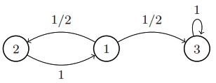
If we start the chain in state 1, it will eventually transition to state 3 and get stuck there.^[State 3 is what is known as a sink state.] It’s not necessary to get stuck in a single state. The same problem arises if state 3 has transitions out, as long as they can’t eventually get back to state 1.
State diagram for another reducible finite Markov chain. The chain will eventually get stuck in state 3 and 4 and never exit to visit states 1 or 2 again.
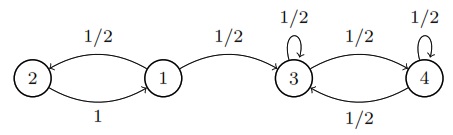
In this example, the chain will eventually fall into a state where it can only visit states 3 and 4.
Periodic chains
A Markov chain can be constructed to cycle through states in a regular (probabilistic) pattern. For example, consider the following Markov chain transitions.
State diagram for finite Markov chain generating periodic state sequences \(\\ldots, 2, 3, 1, 2, 3, 1, 2, 3, 1, 2, \\ldots\).
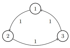
Regular cycles like this defeat the existence of a stationary distribution. If \(Y_1 = 2\), the entire chain is deterministically defined to be
[Y = 2, 3, 1, 2, 3, 1, 2, 3, 1, 2, 3, \ldots.]
Clearly \(p_{Y_t} \neq p_{Y_{t+1}}\), as each concentrates all of its probability mass on a different value.
On the other hand, this chain is what is known as wide-state stationary in that using long-running frequency estimates are stable. The expected value is \(\frac{1 + 2 + 3}{3} = 2\) and the standard deviation is \(\sqrt{\frac{1^2 + 0^2 + 1^2}{3}} \approx 0.47\). More formally, the wide-state expectation is calculated as
[\lim_{T \rightarrow \infty}
\frac{1}{T}
\sum_{t=1}^T Y_t
\rightarrow 2.]
The definition of periodicity is more subtle than just deterministic chains. For example, the following transition graph is also periodic.
State diagram for finite Markov chain generating periodic state sequences alternating between state 1 and either state 2 or state 3.
Rather than a deterministic cycle, it cycles between the state 1 and the pair of states 2 and 3. A simulation might look like
[y^{(1)} = 1, 2, 1, 2, 1, 2, 1, 3, 1, 3, 1, 2, 1, 3, 1, 2, \ldots]
Every other value is a 1, no matter whether the chain starts in state 1, 2, or 3. Such behavior means there’s no stationary distribution. But there is a wide-sense stable probability estimate for the states, namely 50% of the time spent in state 1, and 25% of the time spent in each of states 2 and 3.
Convergence of finite-state chains
In applied statistics, we proceed by simulation, running chains long enough that they provide stable long-term frequency estimates. These stable long-term frequency estimates are of the stationary distribution \(\mbox{categorical}(\pi)\). All of the Markov chains we construct to sample from target distributions of interest (e.g., Bayesian posterior predictive distributions) will be well-behaved in that these long-term frequency estimates will be stable, in theory.^[In practice, we will have to be very careful with diagnostics to avoid poor behavior due to floating-point arithmetic combined with approximate numerical algorithms.]
In practice, none of the Markov chains we employ in calculations will be stationary for the simple technical reason that we don’t know the stationary distribution ahead of time and thus cannot draw \(Y_1\) from it.^[In the finite case, we actually can calculate it either through simulation or as the eigenvector of the transition matrix with eigenvalue one (which is guaranteed to exist). An eigenvector of a matrix is a row vector \(\pi\) such that \(c \times \pi = \theta \, \pi,\) where \(c\) is the eigenvalue. This is why Google’s PageRank algorithm is known to computational statisticians as the “billion dollar eigenvector.” One way to calculate the relevant eigenvector of a stochastic matrix is by raising it to a power, starting from any non-degenerate initial simplex vector \(\lambda\), \(\lim_{n \rightarrow \infty} \lambda \, \theta^n = \pi.\) Each \(\theta^n = \underbrace{\theta \times \theta \times \cdots \times \theta}_{\textstyle n \ \mbox{times}}\) is a transition matrix corresponding to taking \(n\) steps in the original transition matrix \(\theta\).] What we need to know is conditions under which a Markov chain will “forget” its initial state after many steps and converge to the stationary distribution.
All of the Markov chains we will employ for applied statistics applications will be well behaved in the sense that when run long enough, the distribution of each element in the chain will approach the stationary distribution. Roughly, when \(t\) is large enough, the marginal distribution \(p_{Y_t}\) stabilizes to the stationary distribution. The well-behavedness conditions required for this to hold may be stated as follows
Fundamental Convergence Theorem. If a Markov chain \(Y = Y_1, Y_2, \ldots\) is (a) irreducible, (b) aperiodic, and (c) has a stationary distribution \(\mbox{categorical}(\pi)\), then
[\lim_{t \rightarrow \infty}
P_{Y_t}(u) \rightarrow \mbox{categorical}(u \mid \pi).]
What this means in practice is that we can use a single simulation,
[y^{(1)}
\ =
y^{(1)}_1, y^{(1)}_2, \ldots, y^{(1)}_T]
to estimate the parameters for the stationary distribution. More specifically, if we define \(\pi\) by
[\widehat{\pi}_i
\frac{1}{T} \sum_{t = 1}^T \mathrm{I}[y_t^{(1)} = i]]
then we can estimate the stationary distribution as \(\mbox{categorical}(\widehat{\pi}).\)
As a coherence check, we often run a total of \(M\) simulations of the first \(T\) values of the Markov chain \(Y\).
[\begin{array}{rcl} y^{(1)} & = & y_1^{(1)}, y_2^{(1)}, \ldots, y_T^{(1)} \[4pt] y^{(2)} & = & y_1^{(2)}, y_2^{(2)}, \ldots, y_T^{(2)} \[2pt] \vdots \[2pt] y^{(M)} & = & y_1^{(M)}, y_2^{(M)}, \ldots, y_T^{(M)} \end{array}]
We should get the same estimate from using \(y^{(m)}\) from a single simulation \(m\) as we get from using all of the simulated chains \(y^{(1)}, \ldots, y^{(M)}\).^[We’d expect lower error from using all of the chains as we have a larger sample with which to estimate.]
How fast is convergence?
The fundamental theorem tells us that if a Markov chain \(Y = Y_1, Y_2, \ldots\) is ergodic (aperiodic and irreducible) and has a stationary distribution, then the distribution of \(Y_t\) converges to the stationary distribution in the limit. But it doesn’t tell us how fast.
As with everything else, we’ll go at this by simulation to establish intuitions. In particular, we’ll consider three chains that have \(\mbox{bernoulli}(0.5)\) as their stationary distribution (a fair coin toss).
First, we will consider a Markov chain producing independent Bernoulli draws.
State diagram for finite Markov chain generating independent draws.
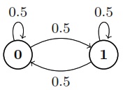
Whether it is currently in state 0 or state 1, there is a 50% chance the next state is 0 and a 50% chance it is 1. Thus each element of the process is generated independently and is identically distributed,
[Y_t \sim \mbox{bernoulli}(0.5).]
Therefore, the stationary distribution must also be \(\pi = (0.5, 0.5)\), because
[\begin{array}{rcl} \pi_1 & = & \pi_1 \times \theta_{1, 1} + \pi_2 \times \theta_{2, 1} \[4pt] 0.5 & = & 0.5 \times 0.5 + 0.5 \times 0.5 \end{array}]
and
[\begin{array}{rcl} \pi_2 & = & \pi_1 \times \theta_{1, 2} + \pi_2 \times \theta_{2, 2} \[4pt] 0.5 & = & 0.5 \times 0.5 + 0.5 \times 0.5. \end{array}]
We can simulate 100 values and print the first 99 to see what the chain looks like.
import numpy as np
import pandas as pd
import matplotlib.pyplot as plt
import seaborn as sns

def print_3_rows_of_33(y):
    n = 0
    for i in range(3):
        row = [str(j) for j in y[n:n+33]]
        print(" ".join(row))
        n += 33

def sample_chain(M, init_state, theta):
    y = [init_state]
    for m in range(1, M):
        y.append(np.random.choice([0, 1], size=1, p=theta[y[m-1], :])[0])
    return y

def traceplot_bool(y):
    df = pd.DataFrame({'iteration': range(1, len(y)+1), 'draw': y})
    plot = sns.lineplot(data=df, x='iteration', y='draw')
    plot.set(xlabel='iteration', ylabel='y', xticks=[1, 50, 100])
    return plot
import numpy as np

np.random.seed(1234)

M = 100
theta = np.array([[0.5, 0.5], [0.5, 0.5]])
y = sample_chain(M, 1, theta)

print_3_rows_of_33(y)
1 0 1 0 1 1 0 0 1 1 1 0 1 1 1 0 1 1 0 1 1 0 1 0 0 1 1 0 1 0 1 1 0
1 0 1 1 0 1 0 1 0 0 0 1 1 1 0 1 0 1 0 1 1 0 1 1 1 1 1 1 0 1 0 0 0
0 0 1 0 0 1 1 0 0 0 1 0 1 0 0 0 1 1 1 1 0 1 1 1 0 0 1 1 1 0 1 1 1
An initial segment of a Markov chain \(Y = Y_1, Y_2, \ldots, Y_T\) can be visualized as a traceplot, a line plot of the value at each iteration.
Traceplot of chain producing independent draws, simulated for 100 time steps. The horizontal axis is time (\(t\)) and the vertical axis the value of e iteration number and the value is the value (\(Y_t\)).
import pandas as pd
import seaborn as sns
import matplotlib.pyplot as plt

def traceplot_bool(y):
    df = pd.DataFrame({'iteration': range(1, len(y)+1), 'draw': y})
    plot = sns.lineplot(data=df, x='iteration', y='draw')
    plot.set(xlabel='iteration', ylabel='y', xticks=[0, 50, 100])
    return plot

traceplot_bool(y)
plt.show()
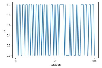
The flat segments are runs of the same value. This Markov chain occasionally has runs of the same value, but otherwise mixes quite well between the values.
So how fast do estimates of the stationary distribution based on an initial segment \(Y_1, \ldots, Y_T\) converge to \(\frac{1}{2}\)? Because each \(Y_t\) is independent and identically distributed, the central limit theorem tells us that the rate of convergence, as measured by standard deviation of the distribution of estimates, goes down as \(\frac{1}{\sqrt{T}}\) with an initial segment \(Y_1, \ldots, Y_T\) of the chain goes down in error as \(\sqrt{T}\)
Now consider a Markov chain which is still symmetric in the states, but with a tendency to stay in the same state.
State diagram for correlated draws.
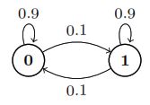
It has the same stationary distribution of 0.5. Letting \(\theta = \begin{bmatrix}0.9 & 0.1 \\ 0.1 & 0.9 \end{bmatrix}\) be the transition matrix and \(\pi = (0.5, 0.5)\) be the probabilities of the stationary distribution we see that the general formula is satisfied by this Markov chain,
[\begin{array}{rcl} \pi_1 & = & \pi_1 \times \theta_{1, 1} + \pi_2 \times \theta_{2, 1} \[4pt] 0.5 & = & 0.5 \times 0.9 + 0.5 \times 0.1 \end{array}]
The same relation holds for \(\pi_2\),
[\begin{array}{rcl} \pi_2 & = & \pi_1 \times \theta_{1, 2} + \pi_2 \times \theta_{2, 2} \[4pt] 0.5 & = & 0.5 \times 0.1 + 0.5 \times 0.9 \end{array}]
We can simulate from the chain and print the first 99 values, and then print the traceplot.
import numpy as np

np.random.seed(1234)

M = 100
theta = np.array([[0.9, 0.1], [0.1, 0.9]])
y = sample_chain(M, 1, theta)

print_3_rows_of_33(y)
1 1 1 1 1 1 1 1 1 1 1 1 1 1 1 1 1 1 0 0 0 0 0 0 0 1 1 1 1 1 1 1 1
1 1 1 1 1 1 1 1 0 0 0 0 0 0 0 0 0 0 0 0 0 0 0 1 1 1 1 1 1 1 1 1 1
0 0 1 1 1 1 1 1 1 1 1 1 1 0 0 0 0 1 1 1 1 1 1 1 1 1 1 1 1 1 1 1 1
Traceplot for chain with correlated draws.”
traceplot_bool(y)
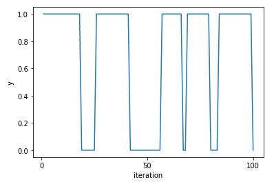
As expected, there are now long runs of the same value being produced. This leads to much poorer mixing and a longer time for estimates based on the draws to converge.
Finally, we consider the opposite case of a symmetric chain that favors moving to a new state each time step.
State diagram for anticorrelated draws.
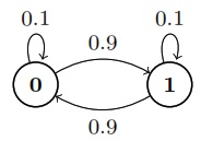
Sampling, printing, and plotting the values produces
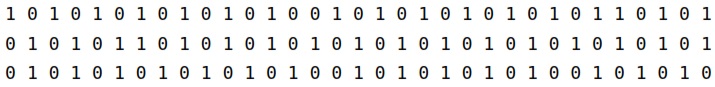
Chain with anticorrelated draws.
import numpy as np

np.random.seed(1234)

M = 100
theta = np.array([[0.1, 0.9], [0.9, 0.1]])
y = sample_chain(M, 1, theta)

print_3_rows_of_33(y)
1 0 1 0 1 0 1 0 1 1 0 1 0 1 0 1 0 1 0 1 0 1 0 0 1 1 0 1 0 1 0 1 0
1 0 1 0 1 1 0 1 0 1 0 1 0 1 0 1 0 1 0 1 0 0 1 1 0 1 1 0 1 0 1 0 1
0 1 1 0 1 0 1 0 1 0 1 0 1 0 1 0 1 1 0 1 0 1 0 1 0 1 0 1 1 0 1 0 1
Traceplot of chain with anticorrelated draws.
traceplot_bool(y)
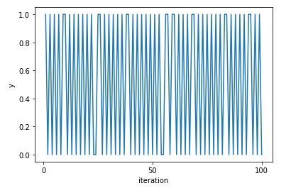
The draws form a dramatic sawtooth pattern as they alternate between zero and one.
Now let’s see how quickly estimates based on long-run averages from the chain converge in a side-by-side comparison. A single chain is enough to illustrate the dramatic differences.
import numpy as np
import pandas as pd

np.random.seed(1234)

def sample_chain(M, start, trans_matrix):
    chain = np.zeros(M, dtype=int)
    chain[0] = start
    for i in range(1, M):
        chain[i] = np.random.choice([0, 1], p=trans_matrix[chain[i-1], :])
    return chain

def build_discrete_mcmc_df(trans_matrix, label, J, M):
    df = pd.DataFrame({'y': [], 'x': [], 'chain': [], 'id': []})
    for j in range(1, J+1):
        y = np.cumsum(sample_chain(M, 1, trans_matrix)) / np.arange(1, M+1)
        df = pd.concat([df, pd.DataFrame({'y': y, 'x': np.arange(1, M+1), 'chain': np.repeat(label, M), 'id': np.repeat(j, M)})])
    return df

corr_trans = np.array([[0.9, 0.1], [0.1, 0.9]])
ind_trans = np.array([[0.5, 0.5], [0.5, 0.5]])
anti_trans = np.array([[0.1, 0.9], [0.9, 0.1]])

J = 25
M = int(1e4)
df_compare_discrete_mcmc = pd.concat([build_discrete_mcmc_df(corr_trans, 'correlated', J, M),
                                      build_discrete_mcmc_df(ind_trans, 'independent', J, M),
                                      build_discrete_mcmc_df(anti_trans, 'anticorrelated', J, M)])
Estimate of the stationary probability \(\pi_1\) of state 1 as a function of \(t\) under three conditions, correlated, independent, and anticorrelated transitions. For each condition, 25 simulations of a chain of size \(T = 10,000\) are generated and overplotted.
import numpy as np
import pandas as pd
from plotnine import *

np.random.seed(1234)

def sample_chain(M, start_state, trans_matrix):
    chain = np.zeros(M)
    chain[0] = start_state
    for i in range(1, M):
        chain[i] = np.random.choice([0, 1], p=trans_matrix[int(chain[i-1]), :])
    return chain

def build_discrete_mcmc_df(trans_matrix, label, J, M):
    df = pd.DataFrame(columns=['y', 'x', 'chain', 'id'])
    for j in range(J):
        y = np.cumsum(sample_chain(M, np.random.choice([0, 1]), trans_matrix)) / (1 + np.arange(M))
        df = pd.concat([df, pd.DataFrame({'y': y, 'x': 1+np.arange(M), 'chain': [label]*M, 'id': [j]*M})])
    return df

corr_trans = np.array([[0.9, 0.1], [0.1, 0.9]])
ind_trans = np.array([[0.5, 0.5], [0.5, 0.5]])
anti_trans = np.array([[0.1, 0.9], [0.9, 0.1]])

J = 25
M = int(1e4)

df_compare_discrete_mcmc = pd.concat([
    build_discrete_mcmc_df(corr_trans, 'correlated', J, M),
    build_discrete_mcmc_df(ind_trans, 'independent', J, M),
    build_discrete_mcmc_df(anti_trans, 'anticorrelated', J, M)
])

compare_discrete_mcmc_plot = (
    ggplot(df_compare_discrete_mcmc, aes(x='x', y='y', group='id')) +
    geom_hline(yintercept=0.5, linetype='dotted', size=0.5) +
    facet_wrap('chain', ncol=1) +
    geom_line(alpha=0.4, size=0.15) +
    scale_x_log10(limits=[100, 10000], breaks=[1e2, 1e3, 1e4], labels=['100', '1,000', '10,000']) +
    scale_y_continuous(limits=[0.25, 0.75], breaks=[0.25, 0.5, 0.75], labels=['.25', '.50', '.75']) +
    xlab('t') +
    ylab('estimated ' + r'$\pi_1$') +
    theme_gray() +
    theme(panel_spacing_y=1)
)
compare_discrete_mcmc_plot
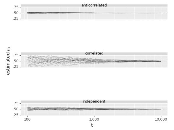
Reversibility
These simple Markov chains wind up being reversible, in that the probability of being in a state \(i\) and then transitioning to state \(j\) is the same as that of being in state \(j\) and transitioning to state \(i\). In symbols, a discrete-valued Markov chain \(Y = Y_1, Y_2, \ldots\) is reversible with respect to \(\pi\) if
[\pi_i \times \theta_{i, j}
\ =
\pi_j \times \theta_{j, i}.]
Reversibility is sufficient for establishing the existence of a stationary distribution.^[If a discrete Markov chain is reversible with respect to \(\pi\), then \(\pi\) is also the unique stationary distribution of the Markov chain.] Markov chains can have stationary distributions without being reversible.^[The reducible chains with we saw earlier are examples with stationary distributions that are not reversible.] But all of the Markov chains we consider for practical applications will turn out to be reversible.
1. Find the stationary distribution \(p_{0}^{0}, p_{1}^{0},\ldots\) for the Markov chain whose only nonzero transition probabilities are:
\(p_{j1} = \frac{j}{j+1},p_{j,j+1} = \frac{1}{j+1} (j = 1, 2,\ldots)\).
Solution
We can find the stationary distribution of the Markov chain by solving the system of equations:
\(\begin{aligned} p_0 &= p_0 \cdot \frac{1}{2} \\ p_j &= p_{j-1} \cdot \frac{j}{j+1} + p_j \cdot \frac{1}{j+1}, \quad j \geq 1 \end{aligned}\)
The first equation simply states that the probability of being in state 0 does not change, since there are no transitions out of state 0.
The second equation can be derived from the law of total probability:
the probability of being in state \(j\) can either come from being in state \(j-1\) and transitioning to state \(j\), or from already being in state \(j\) and staying there.
Solving for the first equation gives \(p_0 = 1\), since any constant multiple of the equation is also a solution.
For the second equation, we can simplify it by multiplying both sides by \((j+1)\) and rearranging:
\(p_{j-1} = \frac{j+1}{j} p_j, \quad j \geq 1\)
We can use this equation to express \(p_j\) in terms of \(p_{j-1}\) recursively:
\(\begin{aligned} p_1 &= p_0 \cdot \frac{1}{2} = \frac{1}{2} \\ p_2 &= \frac{2}{3} p_1 = \frac{1}{3} \\ p_3 &= \frac{3}{4} p_2 = \frac{1}{4} \\ & \cdots \\ p_j &= \frac{1}{j+1} p_{j-1} \end{aligned}\)
We can see that \(p_j = \frac{1}{j+1}\) for all \(j \geq 0\), which is the stationary distribution of the Markov chain.
2. Two gamblers \(A\) and \(B\) repeatedly play a game such that \(A's\) probability of winning is \(p\), while \(B's\) probability of winning is \(q = 1 - p\). Each bet is a dollar, and the total capital of both players is \(m\) dollars. Find the probability of each player being ruined, given that \(A's\) initial capital is \(j\) dollars.
Hint. Let \(e\), denote the state in which \(A\) has \(j\) dollars. Then the situation is described by a Markov chain whose only nonzero transition probabilities are: \(P_{00} = 1, P_{mm} = 1, P_{j,j+1}=p, P_{j,j+1}=q\) \((j = 1, \ldots , m -1)\).
Solution
Let e denote the state in which A has j dollars. We can describe the situation using a Markov chain with m+1 states, where state i represents the situation where A has i dollars. The transition probabilities are given by:
\(P_{i,i+1} = p\), for \(i = 0,1,...,j-1\)
\(P_{i,i+1} = q\), for \(i = j,j+1,...,m-1\)
\(P_{0,0} = P_{m,m} = 1\)
\(P_{i,j} = 0\) for all other \(i,j\)
Note that \(P_{0,0}\) and \(P_{m,m}\) are absorbing states, since once either player has lost all their money, the game ends.
To find the probability of each player being ruined, we can find the probability of reaching the absorbing states starting from state e. Let \(P_i\) denote the probability of reaching the absorbing state \(0\) starting from state \(i\), and \(Q_i\) denote the probability of reaching the absorbing state \(m\) starting from state \(i\).
We can set up a system of equations to solve for \(P_i\) and \(Q_i\):
\(P_{j} = p P_{j+1} + q P_{j-1}\)
\(Q_{j} = p Q_{j+1} + q Q_{j-1}\)
\(P_{0} = 1, P_{m} = 0\)
\(Q_{0} = 0, Q_{m} = 1\)
The first two equations represent the law of total probability: the probability of reaching the absorbing state from state \(j\) can either come from winning the next game and moving to state \(j+1\), or losing the next game and moving to state \(j-1\). The last two equations represent the boundary conditions: the probability of reaching the absorbing state is \(1\) if you are already in the absorbing state, and 0 otherwise.
We can solve for \(P_i\) and \(Q_i\) using standard techniques for solving linear systems of equations. The solution is:
\(P_i = (1 - (q/p)^j (p/q)^{m-j}) / (1 - (q/p)^m)\)
\(Q_i = (1 - (p/q)^{m-j} (q/p)^j) / (1 - (p/q)^m)\)
These formulas give the probability of each player being ruined, depending on their initial capital \(j\) and the total capital \(m\). Note that if \(p = q = 1/2\), then \(P_i = Q_i\) for all \(i\), since the game is fair and both players have the same chance of winning.
3. In the preceding problem, prove that if \(p > q\), then \(f's\) probability of ruin increases if the stakes are doubled.
Solution
Suppose that \(p > q\). Let \(P_j\) and \(Q_j\) denote the probabilities of ruin for A and B, respectively, when the stakes are $1.
Let \(P'_j\) and \(Q'_j\) denote the probabilities of ruin for \(A\) and \(B\), respectively, when the stakes are $2.
We can see that if A is ruined when the stakes are $1, then A will also be ruined when the stakes are $2.
This is because if A is ruined when the stakes are $1, then A has lost all of their money, which means that they would also lose all of their money if the stakes were doubled.
On the other hand, if A is not ruined when the stakes are $1, then A has some positive probability of winning and eventually reaching the total capital of $m.
When the stakes are doubled, A’s probability of winning each game is still p, but the amount of money that A wins in each game is now $2 instead of $1.
This means that A has a higher expected return on each bet, which increases their chances of reaching the total capital of $m.
Therefore, we can see that \(P'_j <= P_j\) for all \(j\), since if A is ruined when the stakes are $1, then A will also be ruined when the stakes are $2, and if A is not ruined when the stakes are $1, then A’s probability of ruin is lower when the stakes are $2.
Similarly, we can see that \(Q'_j >= Q_j\) for all j, since B’s probability of ruin is higher when the stakes are $2.
Therefore, we can conclude that if \(p > q\), then A’s probability of ruin increases if the stakes are doubled.
4. Prove that a gambler playing against an adversary with unlimited capital is certain to be ruined unless his probability of winning in each play of the game exceeds \(\frac{1}{2}\).
Solution
Suppose that a gambler playing against an adversary with unlimited capital has a probability of winning in each play of the game that is less than or equal to \(\frac{1}{2}\). We will prove that the gambler is certain to be ruined.
Let p be the gambler’s probability of winning in each play, and let \(q = 1 - p\) be the adversary’s probability of winning in each play.
Assume that the gambler starts with a capital of j dollars, and that each bet is for one dollar.
Let \(P_j\) denote the probability that the gambler is ruined starting with j dollars.
Suppose that the gambler has j dollars and plays until they are either ruined or have a total capital of m dollars.
Let \(X_k\) denote the gambler’s capital after the \(k^{th}\) bet, and let \(Y_k\) denote the adversary’s capital after the \(k^{th}\) bet. Then we have:
\(X_{k+1} = X_k + 1\) with probability \(p\)
\(X_{k+1} = X_k - 1\) with probability \(q\)
\(Y_{k+1} = Y_k - 1\) with probability \(p\)
\(Y_{k+1} = Y_k + 1\) with probability \(q\)
Note that \(X_k - Y_k\) is a martingale, since the expected value of \(X_{k+1} - Y_{k+1}\) given \(X_k - Y_k\) is equal to \(X_k - Y_k\).
This follows from the fact that the expected value of each of the four possible outcomes for \(X_{k+1} - Y_{k+1}\) given \(X_k - Y_k\) is \(X_k - Y_k\).
Let T denote the first time at which the gambler is ruined or has a total capital of m dollars.
Note that T is a stopping time with respect to the sequence of random variables \(X_0, X_1, ..., X_T\) and \(Y_0, Y_1, ..., Y_T\).
Therefore, we can apply the optional stopping theorem to obtain:
\(j - P_j = E[X_T - Y_T] = E[X_0 - Y_0] = 0\)
This implies that \(P_j = j\), which means that the gambler is certain to be ruined.
Therefore, we can conclude that a gambler playing against an adversary with unlimited capital is certain to be ruined unless their probability of winning in each play of the game exceeds \(\frac{1}{2}\).
Key Points
Discrete Markov Chains
Overview
Teaching: min
Exercises: minQuestions
Objectives
Infinite Discrete Markov Chains
All of the Markov chains we have until now have had a finite number of states. In this chapter, we consider Markov chains with a countably infinite number of states. That is, they are still discrete, but can take on arbitrary integer values.
Drunkard’s walk
The so-called drunkard’s walk is a non-trivial Markov chain which starts with value 0 and moves randomly right one step on the number line with probability \(\theta\) and left one step with probability \(1 - \theta\).
The initial value is required to be zero,
[p_{Y_1}(y_1) \ = \ 1 \ \mbox{ if } \ y_1 = 0.]
Subsequent values are generating with probability \(\theta\) of adding one and probability \(1 - \theta\) of subtracting one,
[p_{Y_{t+1} \mid Y_t}(y_{t+1} \mid y_t)
\ =
\begin{cases}
\theta & \mbox{if } \ y_{t + 1} = y_t + 1, \mbox{and}
[4pt]
1 - \theta & \mbox{if } \ y_{t + 1} = y_t - 1.
\end{cases}]
Another way to formulate the drunkard’s walk is by setting \(Y_1 = 0\) and setting subsequent values to
[Y_{t+1} = Y_t + 2 \times Z_t - 1.]
where \(Z_t \sim \mbox{bernoulli}(\theta).\) Formulated this way, the drunkard’s walk \(Y\) is a transform of the Bernoulli process \(Z\). We can simulate drunkard’s walks for \(\theta = 0.5\) and \(\theta = 0.6\) and see the trend over time.
import numpy as np

M = 10  # Set M to any value you need
theta = 0.5  # Set theta to any value you need
y = np.zeros(M)  # Initialize y with zeros
z = np.zeros(M)  # Initialize z with zeros
y[0] = 0  # Set the first value of y to 0

# Generate z and y values using the Bernoulli distribution
for m in range(1, M):
    z[m] = np.random.binomial(1, theta)
    y[m] = y[m - 1] + (1 if z[m] == 1 else -1)
We’ll simulate from both processes for \(M = 1000\) steps and plot.
Drunkard’s walks of 10,000 steps with equal chance of going left or right (blue) versus a sixty percent chance of going left (red). The dotted line is drawn at the starting point. As time progresses, the biased random walk drifts further and further from its starting point.
import numpy as np
import pandas as pd
import matplotlib.pyplot as plt
import seaborn as sns

np.random.seed(1234)
M = 10000
z1 = np.random.binomial(1, 0.5, M)
z2 = np.random.binomial(1, 0.6, M)
y1 = np.cumsum(2*z1 - 1)
y2 = np.cumsum(2*z2 - 1)

drunkards_df = pd.DataFrame({
    'x': np.concatenate([np.arange(1, M+1), np.arange(1, M+1)]),
    'y': np.concatenate([y1, y2]),
    'drunkard': np.concatenate([np.repeat('50% up / 50% down', M),
                                 np.repeat('60% up / 40% down', M)])
})

drunkards_plot = sns.lineplot(x='x', y='y', hue='drunkard', data=drunkards_df, palette='colorblind')

drunkards_plot.set_xscale('log')
drunkards_plot.set_xlabel('time')
drunkards_plot.set_ylabel('position')
drunkards_plot.set_title('Drunkards Walk')

# Set the legend labels
drunkards_plot.legend(title='Drunkard', labels=['50% up / 50% down', '60% up / 40% down'])

plt.show()
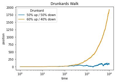
For the balanced drunkard, the expected drift per step is zero as there is equal chance of going in either direction. After 10,000 steps, the expected position of the balanced drunkard remains the origin.^[Contrary to common language usage, the expected position being the origin after \(10,000\) steps does not imply that we should expect the drunkard to be at the origin. It is in fact very unlikely that the drunkard is at the origin after 10,000 steps, as it requires exactly 5,000 upward steps, the probability of which is \(\mbox{binomial}(5,000 \mid 10,000, 0.5) = 0.008.\)] For the unbalanced drunkard, the expected drift per step is \(0.6 \times 1 + 0.4 \times -1 = 0.2\). Thus after 10,000 steps, the drunkard’s expected position is \(0.2 \times 10,000 = 2,000.\)
Gambler’s Ruin
Another classic problem which may be understood in the context of an infinite discrete Markov chain is the gambler’s ruin. Suppose a gambler sits down to bet with a pile of \(N\) chips and is playing a game which costs one chip to play and returns one chip with a probability of \(\theta\).^[The original formulation of the problem, involving two gamblers playing each other with finite stakes, was analyzed in Christiaan Huygens. 1657. Van Rekeningh in Spelen van Geluck. Here we assume one player is the bank with an unlimited stake.] The gambler is not allowed to go into debt, so if the gambler’s fortune ever sinks to zero, it remains that way in perpetuity. The results of the bets at times \(t = 1, 2, \ldots\) can be modeled as an independent and identically distributed random process \(Z = Z_1, Z_2, \ldots\) with
[Z_t \sim \mbox{bernoulli}(\theta).]
As usual, a successful bet is represented by \(Z_t = 1\) and an unsuccessful one by \(Z_t = 0\). The gambler’s fortune can now be defined recursively as a time series \(Y = Y_1, Y_2, \ldots\) in which the initial value is given by
[Y_1 = N]
with subsequent values defined recursively by
[Y_{n + 1}
\ =
\begin{cases}
0 & \mbox{if} \ Y_n = 0, \ \mbox{and}
[4pt]
Y_n + Z_n & \mbox{if} \ Y_n > 0.
\end{cases}]
Broken down into the language of Markov chains, we have an initial distribution concentrating all of its mass at the single point \(N\), with mass function
[p_{Y_1}(N) = 1.]
Each subsequent variable’s probability mass function is given by
[p_{Y_{t + 1} \mid Y_t}(y_{t + 1} \mid y_t)
\ =
\begin{cases}
\theta & \mbox{if} \ y_{t + 1} = y_t + 1
[4pt]
1 - \theta & \mbox{if} \ y_{t + 1} = y_t - 1.
\end{cases}]
These mass functions are all identical in that \(p_{Y_{t+n+1} \mid Y_{t + n}} = p_{Y_{t + 1} \mid Y_t}.\) In other words, \(Y\) is a time-homogeneous Markov chain.
We are interested in two questions pertaining to the gambler. First, what is their expected fortune at each time \(t\)? Second, what is the probability that they have fortune zero at time \(t\).^[A gambler whose fortune goes to zero is said to be ruined.] Both of these calculations have simple simulation-based estimates.
Let’s start with expected fortune and look out \(T = 100\) steps. Suppose the chance of success on any given bet is \(\theta\) and their initial fortune is \(N\). The simulation of the gambler’s fortune is just a straightforward coding of the time series.
import numpy as np

# Set initial values
N = 10
T = 100
theta = 0.5
y = np.zeros(T)
z = np.zeros(T)

# Set initial value of y
y[0] = N

# Simulate the process
for t in range(1, T):
    z[t] = np.random.binomial(1, theta)
    y[t] = y[t - 1] + (1 if z[t] else -1)

print(y)
[10. 11. 10.  9. 10.  9. 10.  9. 10. 11. 12. 13. 12. 13. 14. 13. 14. 15.
 14. 13. 14. 15. 14. 13. 12. 11. 10. 11. 12. 11. 12. 13. 12. 11. 12. 11.
 10.  9.  8.  9.  8.  7.  8.  9. 10. 11. 12. 11. 10. 11. 10.  9.  8.  7.
  6.  5.  4.  3.  2.  3.  4.  3.  2.  3.  2.  3.  2.  3.  4.  3.  4.  3.
  2.  3.  4.  5.  4.  3.  2.  1.  2.  3.  4.  5.  4.  3.  2.  3.  4.  5.
  6.  5.  6.  7.  6.  5.  4.  5.  6.  7.]
Now if we simulate that entire process \(M\) times, we can calculate the expected fortune as an average at each time \(t \in 1:T\).
import numpy as np

# Set initial values
N = 10
T = 100
M = 1000
theta = 0.5
y = np.zeros((M, T))
z = np.zeros((M, T))
expected_fortune = np.zeros(T)

# Simulate the process for each m in M
for m in range(M):
    y[m][0] = N
    for t in range(1, T):
        z[m][t] = np.random.binomial(1, theta)
        y[m][t] = y[m][t - 1] + (1 if z[m][t] else -1)

# Calculate expected fortune at each time point
for t in range(T):
    expected_fortune[t] = np.mean(y[:, t])

print(expected_fortune)
[10.     9.976  9.982  9.986  9.97   9.954  9.992 10.006  9.97   9.986
  9.966  9.984  9.924  9.912  9.838  9.836  9.81   9.78   9.822  9.878
  9.868  9.826  9.86   9.848  9.868  9.876  9.824  9.824  9.78   9.776
  9.788  9.824  9.86   9.93   9.896  9.878  9.864  9.886  9.896  9.938
  9.984  9.962  9.932  9.982  9.996  9.978  9.968  9.948  9.952  9.996
 10.032 10.036 10.02   9.976 10.004  9.998  9.988  9.982  9.996 10.046
 10.004  9.978  9.946  9.994  9.974  9.94   9.898  9.838  9.828  9.808
  9.818  9.85   9.852  9.826  9.816  9.81   9.734  9.712  9.732  9.73
  9.726  9.776  9.74   9.748  9.772  9.778  9.772  9.74   9.754  9.7
  9.72   9.73   9.674  9.71   9.696  9.7    9.764  9.788  9.806  9.858]
Let’s run \(M = 10,000\) simulations for \(T = 50\) starting with a stake of \(N = 5\) with several values of \(\theta\) and plot the expected fortunes.
Expected returns for gambler starting with stake \(N\) and having a \(\theta\) chance at each time point of increasing their fortune by 1 and a \(1 - \theta\) chance of reducing their fortune by 1. The horizontal dotted line is at the initial fortune and the dashed line is at zero.
import numpy as np
import pandas as pd
import matplotlib.pyplot as plt
from scipy.stats import bernoulli
from functools import partial
from itertools import product
from tqdm import tqdm

# Define functions
def simulate_fortune(theta, N=5, T=50):
    y = np.empty((T+1,))
    y[0] = N
    for t in range(1, T+1):
        if y[t-1] == 0:
            y[t] = 0
        else:
            y[t] = y[t-1] + np.random.choice([-1, 1], p=[1-theta, theta])
    return y

def expected_fortune(theta, M=10000, N=5, T=50):
    y = np.empty((M, T+1))
    for m in range(M):
        y[m] = simulate_fortune(theta, N=N, T=T)
    return np.mean(y[:, 1:], axis=0)

# Set parameters
np.random.seed(1234)
N = 5
T = 50
M = 10000
Theta = [0.4, 0.5, 0.6]

# Simulate and plot expected fortune
df_ruin = pd.DataFrame(columns=['time', 'expected_fortune', 'theta'])
for theta in Theta:
    expected_fortune_theta = expected_fortune(theta, M=M, N=N, T=T)
    df_theta = pd.DataFrame({'time': range(1, T+1),
                             'expected_fortune': expected_fortune_theta,
                             'theta': ['theta = {}'.format(theta)]*T})
    df_ruin = pd.concat([df_ruin, df_theta])

# Plot
fig, axes = plt.subplots(nrows=1, ncols=3, figsize=(15, 5))
for i, theta in enumerate(Theta):
    df_theta = df_ruin[df_ruin['theta'] == 'theta = {}'.format(theta)]
    ax = axes[i]
    ax.plot(df_theta['time'], df_theta['expected_fortune'])
    ax.axhline(y=N, linestyle=':', color='gray', linewidth=0.5)
    ax.axhline(y=0, linestyle='--', color='gray', linewidth=0.5)
    ax.set_title('theta = {}'.format(theta))
    ax.set_xlabel('time')
    ax.set_ylabel('expected fortune')
    ax.set_xticks([1, 25, 50])
    ax.set_yticks([0, 5, 10, 15])
plt.tight_layout()
plt.show()
Next, we’ll tackle the problem of estimating the probability that a gambler has run out of money at time \(t\). In symbols, we are going to use simulations \(y^{(1)}, \ldots, y^{(M)}\) of the gambler’s time series,
Expected Fortune over Time for Different Values of \(\Theta\)
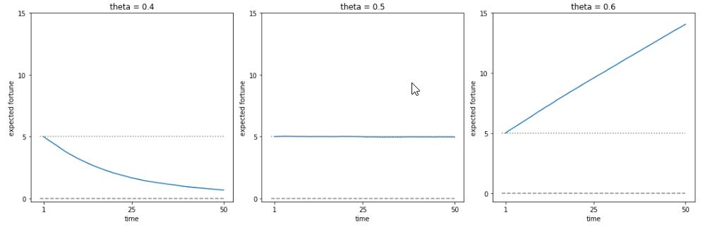
[\begin{array}{rcl} \mbox{Pr}[Y_t = 0] & = & \mathbb{E}\left[ \mathrm{I}\left[ Y_t = 0 \right] \right]. [6pt] & \approx & \displaystyle \frac{1}{M} \sum_{m = 1}^M \, \mathrm{I}\left[ y_t^{(m)} = 0 \right]. \end{array}]
This last term can be directly calculated by adding the indicator variables to the calculations before.
for m in range(M):
    y[m, 0] = N
    for t in range(1, T):
        z = np.random.binomial(1, theta)
        y[m, t] = y[m, t - 1] + (1 if z else -1)
        ruined[m, t] = (y[m, t] == 0)
for t in range(T):
    estimated_pr_ruin[t] = np.mean(ruined[:, t])
So let’s run that and plot the probability of ruin for the same three choices of \(\theta\), using \(M = 5,000\) simulations. But this time, we’ll run for \(T = 200\) time steps.
Probability of running out of money for a gambler starting with stake \(N\) and having a \(\theta\) chance at each time point of increasing their fortune by 1 and a \(1 - \theta\) chance of reducing their fortune by 1. The horizontal dotted line is at 100 percent.
import numpy as np
import pandas as pd
import seaborn as sns
import matplotlib.pyplot as plt

np.random.seed(1234)

N = 5
T = 200
M = 5000
Theta = [0.4, 0.5, 0.6]

df_expect_ruin = pd.DataFrame(columns=['x', 'y', 'theta'])
for theta in Theta:
    y = np.empty((M, T))
    for m in range(M):
        y[m, 0] = N
        for t in range(1, T):
            if y[m, t - 1] == 0:
                y[m, t] = 0
            else:
                z = np.random.binomial(1, theta)
                y[m, t] = y[m, t - 1] + (1 if z else -1)
    pr_ruin = np.mean(y == 0, axis=0)
    df_theta = pd.DataFrame({
        'x': range(1, T+1),
        'y': pr_ruin,
        'theta': [f'theta = {theta}'] * T
    })
    df_expect_ruin = pd.concat([df_expect_ruin, df_theta], ignore_index=True)

sns.set_theme(style="whitegrid")
g = sns.relplot(
    data=df_expect_ruin, x='x', y='y',
    col='theta', kind='line', facet_kws=dict(sharey=False),
    col_wrap=3, height=4, aspect=1.2
)
g.set_axis_labels('time', 'probability of ruin')
g.set(xticks=[1, 100, 200], yticks=[0, 0.25, 0.5, 0.75, 1],
      yticklabels=['0', '1/4', '1/2', '3/4', '1'])
g.fig.subplots_adjust(top=0.85)
g.fig.suptitle('Expectation of ruin over time for different values of theta')
plt.show()
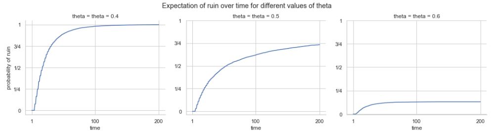
Even in a fair game, after 50 bets, there’s nearly a 50% chance that a gambler starting with a stake of 5 is ruined; this probabiltiy goes up to nearly 75% after 200 bets.
Queueing
Suppose we have a checkout line at a store (that is open 24 hours a day, 7 days a week) and a single clerk. The store has a queue, where customers line up for service. The queue begins empty. Each hour a random number of customers arrive and a random number of customers are served. Unserved customers remain in the queue until they are served.
To make this concrete, suppose we let \(U_t \in 0, 1, \ldots\) be the number of customers that arrive during hour \(t\) and that it has a binomial distribution,
[U_t \sim \mbox{binomial}(1000, 0.005).]
Just to provide some idea of what this looks like, here are 20 simulated values,
import numpy as np

M = 20
y = np.random.binomial(n=1000, p=0.005, size=M)

for m in range(M):
    print(f"{y[m]:2.0f}", end=" ")
6 7 6 9 8 8 5 5 7 2 2 4 5 7 5 0 3 2 6 4
We can think of this as 1000 potential customers, each of which has a half percent chance of deciding to go to the store any hour. If we repeat, the mean number of arrivals is 5 and the standard deviation is 2.2.
Let’s suppose that a clerk can serve up to \(V_t\) customers per hour, determined by the clerk’s rate \(\phi\),
[V_t \sim \mbox{binomial}(1000, \phi).]
If \(\phi < 0.005,\) there is likely to be trouble. The clerk won’t be able to keep up on average.
The simulation code just follows the definitions.
import numpy as np

queue = np.zeros(T) # Initialize queue array to zeros
queue[0] = 0 # Set first element to 0

for t in range(1, T):
    arrive[t] = np.random.binomial(n=1000, p=0.005)
    serve[t] = np.random.binomial(n=1000, p=phi)
    queue[t] = max(0, queue[t-1] + arrive[t] - serve[t])
The max(0, ...) is to make sure the queue never gets negative. If
the number served is greater than the total number of arrivals and
customers in the queue, the queue starts empty the next time step.
Let’s try different values of \(\phi\), the average server rate, and plot two weeks of service.^[\(24 \mbox{hours/day} \ \times 14 \ \mbox{days} = 336 \mbox{hours}\)]
Multiple simulations of queue size versus time for a queue with \(\mbox{binomial}(1000, 0.005)\) customers arriving per hour (an average of 5), and a maximum of \(\mbox{binomial}(1000, \phi)\) customers served per hour, plotted for various \(\phi\) (as indicated in the row labels).
import numpy as np
import pandas as pd
import matplotlib.pyplot as plt
import seaborn as sns

np.random.seed(1234)

T = 14 * 24
run = 1
queue = np.empty(T)
queue[:] = np.nan

queue_df = pd.DataFrame({'t': [], 'queue': [], 'run': [], 'phi': []})

for m in range(50):
    for phi in [0.005, 0.0055, 0.006, 0.01]:
        queue[0] = 0
        for t in range(1, T):
            arrived = np.random.binomial(n=1000, p=0.005, size=1)
            served = np.random.binomial(n=1000, p=phi, size=1)
            queue[t] = max(0, queue[t-1] + arrived - served)
        df = pd.DataFrame({
            't': range(1, T+1),
            'queue': queue,
            'run': np.repeat(run, T),
            'phi': np.repeat(f'phi = {phi}', T)
        })
        queue_df = pd.concat([queue_df, df])
        run += 1

grid = sns.FacetGrid(queue_df, col='phi', sharey=False)
grid.map(sns.lineplot, 't', 'queue', 'run', alpha=0.2, linewidth=0.9,color='blue')
grid.set(xticks=[1, 100, 200, 300], yticks=[0, 50, 100, 150])
grid.set_axis_labels(x_var='hours open', y_var='queue size')
plt.show()
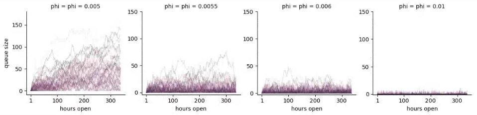
As can be seen in the plot, the queue not growing out of control is very sensitive to the average service rate per hour. At an average rate of five customers served per hour (matching the average customer intake), the queue quickly grows out of control. With as few as five and a half customers served per hour, on average, it becomes stable long term; with seven customers served per hour, things settle down considerably. When the queue goes up to 50 people, as it does with \(\phi = 0.0055\), wait times are over ten hours. Because of the cumulative nature of queues, a high server capacity is required to deal with spikes in customer arrival.
Key Points
Continuous Random Variables
Overview
Teaching: min
Exercises: minQuestions
Objectives
Continuous Random Variables
So far, we have only considered discrete random variables, i.e., variables taking only integer values. But what if we want to use random variables to represent lengths or volumes or distances or masses or concentrations or any of the other continuous properties in the physical world? We will need to generalize our approach so far.
Continuous random variables take on real values. The set of real numbers is uncountable in the sense of being strictly larger than the set of integers.^[Georg Cantor developed the technique of diagonalization to show it was impossible to have a one-to-one map from the reals to the integers, thus proving the set of reals is uncountable.]
The mathematics of probability is the same for real values. Even more importantly from a practical standpoint, the way we calculate event probabilities and estimates remains the same with continuous quantities. The notion of a probability mass function, on the other hand, must be replaced by its continuous equivalent, the probability density function.
Spinners and uniform continuous variables
Suppose \(\Theta\) is a random variable representing the angle at which a fair spin of a spinner lands. We will use degrees and thus suppose the value of \(\Theta\) is between 0 and 360^[The end points are the same, representing a complete rotation of 360 degrees; they are labeled as such in the plot.]
A spinner resting at 36 degrees, or ten percent of the way around the circle. A fair spin might land anywhere between 0 and 360 degrees.
df_spinner <- data.frame(value = c("0-360 degrees"), prob = c(0.3))
plot_spinner <-
  ggplot(data = df_spinner,
         aes(x = factor(1), y = prob, fill = value)) +
  geom_bar(stat = "identity", position = "fill", fill = "#ffffe8",
           color="black", size = 0.25) +
  coord_polar(theta = "y") +
  geom_segment(aes(y =  0.1, yend =  0.1, x = -1, xend = 1.375),
               arrow = arrow(type = "open"),
	       size = 0.5, color = "#666666") +
  geom_point(aes(x = -1, y = 0), color = "#666666", size = 3) +
  scale_x_discrete(breaks = c()) +
  scale_y_continuous(breaks = c(0, 0.1, 0.25, 0.5, 0.75),
                     labels = c("360 | 0    ", "36", "90", "180", "270")) +
  xlab(expression(paste(theta, " degrees"))) +
  ylab("") +
  ggtheme_tufte() +
  theme(legend.position = "none")
plot_spinner
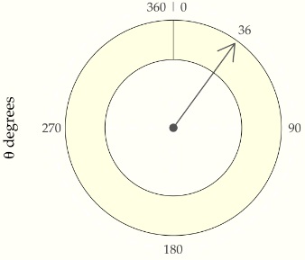
What does fair mean for continuous probabilities? At the least, we should be able to say that the probality of landing in any band is the same no matter where the band lies on the circle. That is, landing between 0 and 36 degrees should be the same as landing between 200 and 236 degrees. Also, because 36 degrees is one tenth of the way around the circle, the chance of landing in any 36 degree band has to be 10%.^[A circle can be divided into ten bands of 36 degrees to create exhaustive and exclusive intervals, the event probabilities of landing in which must be the same by fairness and must total one because they exhaust all possible outcomes.] We can express that in probability notation as
[\mbox{Pr}[0 \leq \Theta \leq 36]
\ =
\frac{1}{10}]
and
[\mbox{Pr}[200 \leq \Theta \leq 236]
\ =
\frac{1}{10}.]
We are not talking about the probability of \(\Theta\) taking on a particular value, but rather of it falling in a particular interval.^[ In general, the probability of a fair spinner \(\Theta\) falling in interval is the fraction of the circle represented by the interval, i.e., \(\mbox{Pr}[\theta_1 \leq \Theta \leq \theta_2] = \frac{\theta_2 - \theta_1}{360}.\) for \(0 \leq \theta_1 \leq \theta_2 \leq 360.\)] For continuous random variables, outcomes do not have probability mass. Instead, probability mass is assigned continuously based on the probability of a variable falling in a region.
The paradox of vanishing point probabilities
In our first example, we took a fair spinner to land at exactly 36 degrees; it could’ve been 36.0376531 degrees or even an irrational number such as \(0.3333\cdots.\)^[When I learned decimal representations, we wrote \(0.\bar{3}\) for the decimal representation of \(\frac{1}{3}.\)] What’s the probability the spinner landed on exactly 36 degrees? Paradoxically, the answer is zero.
[\mbox{Pr}[\Theta = 36] = 0.]
Why must this be? If the probability of any specific outcome was greater than zero, every other possible value would have to have the same probability to satisfy fairness. But then if we summed them all up, the total would be greater than one, which is not possible. Something has to give, and that something is the idea of particular point outcomes having probability mass in a continuous distribution. The paradox arises because some number must come up, but every number has zero probability.
Simulating uniform values
We will assume that our programming language comes equipped with a
function uniform_rng(L, H) that generates numbers uniformly in the
interval \([L, H]\).
For instance, the following program simulates from the uniform interval.
import numpy as np

M = 5  # Number of elements
y = np.zeros(M)  # Initialize the output array with zeros

for m in range(M):
    y[m] = np.random.uniform(0, 1)

print('y =', y)
y = [0.38758361 0.45822924 0.24143984 0.44435819 0.25484211]
Let’s simulate \(M = 10\) draws and look at the result,
 import numpy as np

np.random.seed(1234)  # Set the random seed
M = 10  # Number of elements
y = np.random.uniform(size=M)  # Generate the random array

for m in range(M):
    print(f'{y[m]:5.4f}', end=' ')  # Print each element with format '5.4f'
0.1915 0.6221 0.4377 0.7854 0.7800 0.2726 0.2765 0.8019 0.9581 0.8759
These are only printed to a few decimal places. As usual, it’s hard to get a sense for the sequence of values as raw numbers. The most popular way to summarize one-dimensional data is with a histogram, as shown in the following plot.
Histogram of 10 draws from a \(\\mbox{uniform}(0, 1)\) distribution.
from plotnine import *
import pandas as pd

df_unif_10 = pd.DataFrame({'y': y})
unif_10_plot = ggplot(df_unif_10, aes(x='y')) + \
  geom_histogram(binwidth=0.1, center=0.05, color="black", fill="#ffffe6", size=0.25) + \
  scale_x_continuous(breaks=[i/10 for i in range(0, 11)], limits=[0, 1], expand=[0, 0.02], name="y") + \
  scale_y_continuous(breaks=[1, 2, 3, 4, 5], expand=[0.02, 0], name="count") + \
  theme_tufte()

print(unif_10_plot)
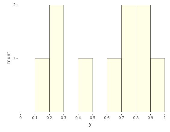
The range of values from 0 to 1 is broken up into ten equally spaced bins, 0 to 0.1, 0.1 to 0.2, up to 0.9 to 1.0. Each bin is then drawn as a rectangle with a height proportional to the number of values that fell into the bin.
Even though the distribution draws uniformly in the interval, with only ten draws, the probability of having one draw in each bin is small,^[The first draw can be in any bin, the second in any of 9 bins, the third in any of 8 bins, and so on, yielding a probability for each bin containing a single draw of \(\prod_{n=1}^{10} \frac{n}{10} \approx 0.00036.\)] whereas the probability of having many values in a single bin is relatively high.^[For example, the probability of having a bin with exactly five draws involves a choice of the distinguished bin, a choice of which of the five draws go in the distinguished bin, then the probabilities of the distinguished bins and other bins, \({10 \choose 1} \times {10 \choose 5} \times \left(\frac{1}{10}\right)^5 \times \left(\frac{9}{10}\right)^5 \approx 0.015.\)] As usual, we turn to repetition and sizing to see what’s going on.
Histograms for uniform(0, 1) samples of increasing sizes. The proportion of draws falling into each bin becomes more uniform as the sample size increases. With each sample plotted to the same height, the vertical count axis varies in scale among the plots.
import pandas as pd
import numpy as np
import matplotlib.pyplot as plt
import seaborn as sns
import plotnine as p9

np.random.seed(1234)
df_unif = pd.DataFrame()
for N in [2**n for n in range(2, 13, 2)]:
    y = np.random.uniform(size=N)
    df_unif = pd.concat([df_unif, pd.DataFrame({'y': y, 'size': ['N={}'.format(N)] * N})])

plot = (
    p9.ggplot(df_unif, p9.aes(x='y')) +
    p9.facet_wrap('size', scales='free') +
    p9.geom_histogram(binwidth=0.1, center=0.05, color='black', fill='#ffffe6') +
    p9.scale_x_continuous(breaks=[0, 0.5, 1], labels=['0.0', '0.5', '1.0'], limits=[0, 1], expand=[0, 0.02]) +
    p9.scale_y_continuous(name='proportion of draws', breaks=[], expand=(0.02, 0)) +
    p9.theme(panel_spacing={'y': 24, 'x': 24}, aspect_ratio=0.5, subplots_adjust={'wspace': 0.25}) +
    p9.theme_tufte()+ theme(subplots_adjust={'hspace': 0.25}))
plot
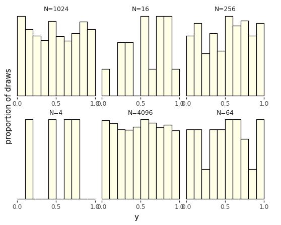
Calculating \(\pi\) via simulation
Now that we have a continuous random number generator, there are all kinds of values we can compute. Here, we show how to calculuate the first few digits of \(\pi\). We’ll carry this out by formulating an event probability over some continuous random variables whose probability is a fraction of \(\pi\).
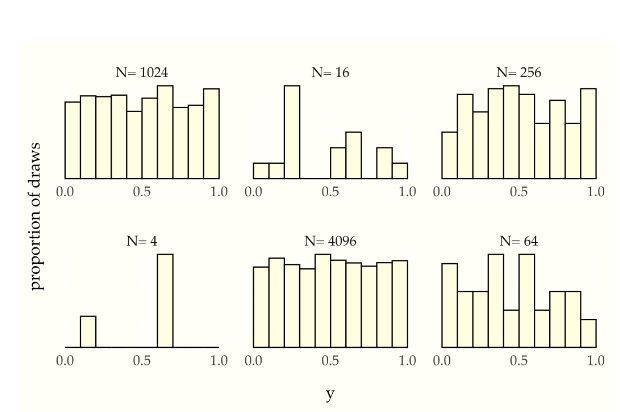 We start with the basic fact of algebra that that \(\pi\) is the area of
a unit radius circle.^[The area of a circle of radius \(r\) is \(\pi
\times r^2\), so when \(r = 1\), the area is \(\pi\).] We then assume there
are two independent, uniform random variables \(X\) and \(Y\),
We start with the basic fact of algebra that that \(\pi\) is the area of
a unit radius circle.^[The area of a circle of radius \(r\) is \(\pi
\times r^2\), so when \(r = 1\), the area is \(\pi\).] We then assume there
are two independent, uniform random variables \(X\) and \(Y\),
[X, Y \sim \mbox{uniform}(-1, 1).]
Simulations \(x^{(m)}, y^{(m)}\) of these variables pick out a point on the plane within a square bounded by -1 and 1 in both dimensions. Here is a plot of the square in which the draws will fall. Also shown is a circle of unit radius inscribed within that square. Draws may or may not fall within the circle.^[Technically, the bearer of area is a disc and the line around its border a circle. Mathematicians are picky because, topologically speaking, a disc has two dimensions whereas a circle has but one.]
A unit circle (dotted line) centered at the origin is inscribed in a square (dashed lines) with axes running from -1 to 1.
import numpy as np
import plotnine as p9
from plotnine.themes import theme_tufte
from numpy import cos
from numpy import sin


radians = np.linspace(0, 2*np.pi, 100)

bullseye_target_plot = (
  p9.ggplot(p9.aes(x='X', y='Y')) +
  p9.geom_path(
    data=p9.aes(x=cos(radians), y='sin(radians)'),
    size=0.8, color='#333333', linetype="dotted"
  ) +
  p9.geom_path(
    data=p9.aes(x=[-1, -1, 1, 1, -1], y=[-1, 1, 1, -1, -1]),
    size=0.4, color='#333333', linetype="dashed"
  ) +
  p9.scale_x_continuous(limits=[-1, 1], breaks=[-1, 0, 1]) +
  p9.scale_y_continuous(limits=[-1, 1], breaks=[-1, 0, 1]) +
  p9.coord_fixed(ratio=1) +
  theme_tufte()
)
bullseye_target_plot
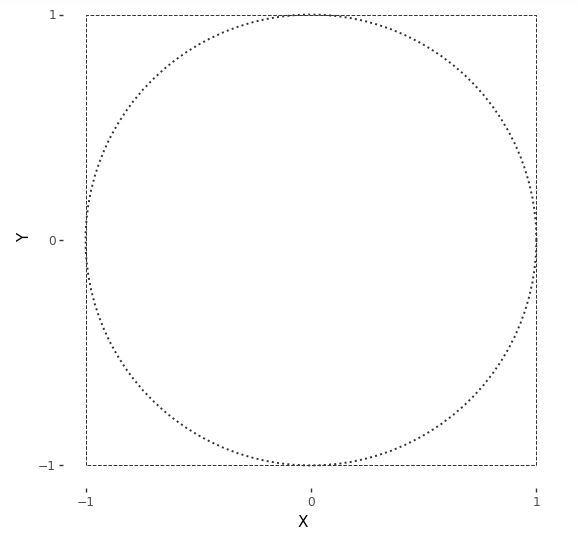
A point \((x, y)\) will fall within the unit circle if^[A point falls on a circle of radius \(r\) if \(x^2 + y^2 = r^2\).]
[x^2 + y^2 \leq 1.]
Let’s see what this looks like with \(M = 250\) draws. The resulting plot is known as a scatterplot—it places values at their \((x, y)\) coordinates, resulting in them being “scattered.”
\(M = 250\) simulated draws of \((x^{(m)}, y^{(m)})\) from a \(\\mbox{uniform}(-1, 1)\) distribution. Points within the circle are plotted using \(+\) and those outside it with \(\\circ\).
import numpy as np
import pandas as pd
import plotnine as p9
from plotnine.themes import theme_tufte

np.random.seed(1234)

M = 250
X = np.random.uniform(-1, 1, size=M)
Y = np.random.uniform(-1, 1, size=M)
df = pd.DataFrame({'X': X, 'Y': Y, 'within': (X**2 + Y**2 < 1)})

radians = np.linspace(0, 2*np.pi, 200)

bullseye_plot = (
    p9.ggplot(df, p9.aes(x='X', y='Y')) +
    p9.annotate("path", x=np.cos(radians), y=np.sin(radians),
                 size=0.8, color='#333333', linetype="dashed") +
    p9.annotate("path", x=[-1, -1, 1, 1, -1], y=[-1, 1, 1, -1, -1],
                 size=0.4, color='#333333', linetype="dotted") +
    p9.geom_point(p9.aes(shape='within', color='within'), size=2.25) +
    p9.scale_shape_manual(values=[1, 3]) +
    p9.scale_color_manual(values=["blue","red"]) + #"#333333", "#111111"
    p9.scale_x_continuous(limits=[-1, 1], breaks=[-1, 0, 1]) +
    p9.scale_y_continuous(limits=[-1, 1], breaks=[-1, 0, 1]) +
    p9.coord_fixed(ratio=1) +
    theme_tufte() +
    p9.theme(legend_position="none")
)

bullseye_plot
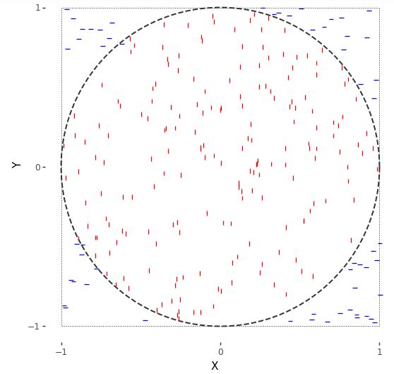
For random variables \(X, Y \sim \mbox{uniform}(-1, 1)\), the event of their falling within the unit circle is \(X^2 + Y^2 \leq 1\). Because \(X\) and \(Y\) are drawn uniformly from within the square, the probability of their being within the circle is proportional to the circle’s area. The circle’s area is \(\pi\), whereas the overall area of the square is 4. So the probability of a random draw within the square being within the circle is
[\mbox{Pr}[X^2 + Y^2 \leq 1] = \frac{\pi}{4}.]
We know how to estimate event probabilities using simulation. The code here is straightforward.
import random

M = 1000000  # set the number of samples
inside = 0  # initialize the counter for points inside the circle

# generate M random points and count how many are inside the circle
for m in range(M):
    x = random.uniform(-1, 1)
    y = random.uniform(-1, 1)
    if x**2 + y**2 <= 1:
        inside += 1

# estimate pi using the number of points inside the circle
pi_estimate = 4 * inside / M

# print the results
print('Pr[in circle] =', inside / M)
print('estimated pi =', pi_estimate)
Pr[in circle] = 0.78507
estimated pi = 3.14028
We recover the simulation-based estimate of \(\pi\) by multiplying the event probability of \(X^2 + Y^2 \leq 1\) by four.
Let’s run this with \(M = 1,000,000\) and see what we get,
import numpy as np

np.random.seed(1234)  # set the random seed
M = 1000000  # set the number of samples
X = np.random.uniform(-1, 1, M)
Y = np.random.uniform(-1, 1, M)
inside = np.sum(X**2 + Y**2 < 1)  # count the number of points inside the circle
Pr_target = inside / M  # compute the target probability

# print the results
print(f"Pr[in circle] = {Pr_target:.3f}")
print(f"estimated pi = {4 * Pr_target:.3f}")
Pr[in circle] = 0.786
estimated pi = 3.143
We actually knew the answer ahead of time here, \(\pi \approx 3.14159\). The simulation-based estimate is on the right track.^[But not going to win any \(\pi\) digit-generating contests, either. Remember, we need one hundred times as many draws for each subsequent digit of precision using i.i.d. simulation.] At least the first couple of digits are correct.
If you want to do this all the old-fashioned way with calculus, note that the top half of the circle is given by the function $$y = \sqrt{1
- x^2}\(. Integrating this from\)-1\(to\)1$$ and doubling it thus produces the required value,
[\pi = 2 \times \int_{-1}^1 \sqrt{1 - x^2} \, \mathrm{d}x.]
Simulation-based methods are largely used in practice to solve nasty integrals without analytic solutions.
The curse of dimensionality
In most introductory examples, including the ones in this book, intuitions are developed based on one or two dimensions—essentially, we use what can be visualized. It turns out that intuitions based on a few dimensions are not only useless, but harmful, when extended to higher dimensions. This section attempts to explain why, and along the way, introduce the key notion for sampling of the typical set.
Working by example, let’s start with the base case of a single random variable \(X_1\) with a uniform distribution over the line in the interval \((0, 1)\),
[X_1 \sim \mbox{uniform}(0, 1).]
The length of our unit line is one (hence the name), so the probability of falling in an interval is proportional to the interval’s length.^[This also explains why a point has probability zero—it has length zero.]
Now extend this to two dimensions, letting the pair of random variables \((X_1, X_2)\) be uniformly distributed in the unit square, \((0, 1) \times (0, 1)\),
[X_1, X_2 \sim \mbox{uniform}(0, 1).]
The area of a \(1 x 1\) square is one, so that the probability of falling in a region within that square is proportional to the area of the region.^[Thus a point or a line has zero probability in a square.]
Going one dimension further, let \((X_1, X_2, X_3)\) be random variables uniformly distributed in a unit cube, \((0, 1)^3 = (0, 1) \times (0, 1) \times (0, 1)\),
[X_1, X_2, X_3 \sim \mbox{uniform}(0, 1).]
The unit cube has unit volume, \(1 \times 1 \times 1 = 1\). Thus the probability of falling in a region within that cube is proportional to the volume of the region.^[Thus a plane has zero probability in a cube. This generalizes in the obvious way, so this will be the last note.]
Now we can just go all the way, and let \(X = (X_1, \ldots, X_N)\) be an \(N\)-dimensional random variable generated uniformly in an \(N\)-dimensional unit hypercube, \((0, 1)^N\),
[X_n \sim \mbox{uniform}(0, 1) \ \ \mbox{for} \ \ n \in 1:N.]
As before, the hypervolume is \(1 \times 1 \times \cdots \times 1 = 1\), so the probability of lying in a region of the hypercube is proportional to the hypervolume of the region.^[The fact that we go from line to square to cube and then run out of words should be a tipoff that we’re barely acquainted with high dimensions. To be fair, we have “tesseract” for a four-dimensional hypercube, but that’s a technical term that might have lain buried in introductions to geometry if not for the Marvel Universe, and even there, it was known colloquially as “the cube.”]
We saw that in two dimensions, the probability of a random draw from a unit square lying in the inscribed circle was approximately 0.74. As dimensionality increases, this number goes to zero quickly. In other words, most of the probability mass (as measured by hypervolume) in high dimensions lies in the corners. Let’s see just how much by simulation.
import numpy as np

def euclidean_length(x):
    return np.sqrt(np.sum(np.square(x)))

max_log2_N = 10
M = 5

mean_d = np.zeros(max_log2_N)
min_d = np.zeros(max_log2_N)
max_d = np.zeros(max_log2_N)

for log2_N in range(1, max_log2_N+1):
    N = 2**log2_N
    d = np.zeros(M)
    for m in range(M):
        x = np.random.uniform(-0.5, 0.5, size=N)
        d[m] = euclidean_length(x)
    mean_d[log2_N-1] = np.mean(d)
    min_d[log2_N-1] = np.min(d)
    max_d[log2_N-1] = np.max(d)
We take x^2 to operate elementwise on the members of x, e.g.,
\((1, 2, 3)^2 = (1, 4, 9)\). The square root, sum, and other operations
should be self explanatory. The Euclidean length function is being
defined with lambda abstraction, where the x. indicates that the
argument to the function is x and the result is the result of
plugging the value for x into the body, sqrt(sum(x^2)).
Let’s plot what we get out to \(1,000\) dimensions or so.
Plot of the average distance (solid line) of a uniform draw from a hypercube to the center of the hypercube as a function of the number of dimensions. The minimum and maximum distance (dotted lines) are shown based on \(M = 10,000\) simulations.
import numpy as np
import pandas as pd
import matplotlib.pyplot as plt

def euclidean_length(x):
    return np.sqrt(np.sum(x**2))

np.random.seed(1234)
M = 10000
log2maxN = 10
min_d = np.empty(log2maxN)
max_d = np.empty(log2maxN)
mean_d = np.empty(log2maxN)
d = np.empty(M)
for log2n in range(1, log2maxN+1):
    n = 2**log2n
    for m in range(M):
        x = np.random.uniform(-0.5, 0.5, size=n)
        d[m] = euclidean_length(x)
    min_d[log2n-1] = np.min(d)
    max_d[log2n-1] = np.max(d)
    mean_d[log2n-1] = np.mean(d)
# print(f'min_d[log2n-1]={min_d},max_d[log2n-1] ={max_d },mean_d[log2n-1]={mean_d}')
df_curse = pd.DataFrame({
    'dimensions': np.repeat(2**np.arange(1, log2maxN+1), 3),
    'distance': np.concatenate((min_d, mean_d, max_d)),
    'type': np.repeat(['min', 'mean', 'max'], log2maxN)
})
# print(df_curse )
curse_plot = (
    ggplot(df_curse, aes(x='dimensions', y='distance')) +
    geom_line(aes(linetype='type'), size=0.5) +
    scale_x_log10(breaks=[1, 10, 100, 1000, 10000]) +
    scale_y_continuous(breaks=[0, 2, 4, 6, 8, 10]) +
    scale_linetype_manual(values=['dotted', 'solid', 'dotted']) +
    ylab('Distance of draw to center') +
    xlab('Dimensions of unit hypercube') +
    theme_tufte() +
    theme(legend_position='none')
)
curse_plot
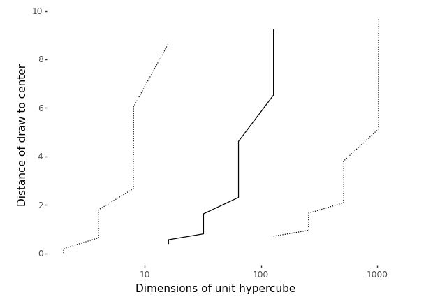
While it may seem intuitively from thinking in two dimensions that draws should be uniformly dispersed and thus appear near the origin, they in fact do two things that are quite surprising based on our low-dimensional intuitions,
- draws get further and further away from the origin, on average, as dimension increases, and
- draws accumulate in a thin shell of distance from the origin, with no draws being anywhere near the origin in high dimensions.
The first fact is obvious when you consider the definition of distance is the square root of the squared dimension values, which we will write as
| [ | x | = \sqrt{x_1^2 + x_2^2 + \cdots + x_N^2}.] |
In this form, it is clear that as \(N\) increases, so does \(||x||\) as we simply keep adding squared terms \(x_n^2\) with each additional dimension.
Although the draws accumulate in a thin shell of distance from the origin, it would be wrong to conclude that they are anywhere near each other. They are further from each other, on average, than they are from the origin. For example, let’s simulate just for 100 dimensions,
import numpy as np

M = 10000
N = 10
d = np.empty(M)
for m in range(M):
    x = np.random.uniform(-0.5, 0.5, size=N)
    y = np.random.uniform(-0.5, 0.5, size=N)
    d[m] = np.sqrt(np.sum((x - y)**2))
print('min =', np.min(d), '; mean =', np.mean(d), '; max =', np.max(d))
min = 0.38514151598863117 ;
mean = 1.2702829208415631 ;
max = 2.1206861405752284
Let’s run that for \(M = 10,000\) and \(N = 100\) and see what we get.
import numpy as np

N = 100
M = 10000
d = np.empty(M)
for m in range(M):
    x = np.random.uniform(size=N)
    y = np.random.uniform(size=N)
    d[m] = np.sqrt(np.sum((x - y)**2))
print(f"min = {np.min(d):.1f}; mean = {np.mean(d):.1f}; max = {np.max(d):.1f}")
min = 3.1; mean = 4.1; max = 5.0
We see that the average distances between randomly generated points is even greater than the average distance to the origin.
Key Points
Continuous Distributions and Densities
Overview
Teaching: min
Exercises: minQuestions
Objectives
Continuous Distributions and Densities
Continuous cumulative distribution functions
Suppose \(\Theta \sim \mbox{uniform}(0, 360)\) is the result of spinning a fair spinner. The cumulative distribution function is defined exactly as for discrete random variables,^[Note that we have moved from Roman to Greek letters, but have kept to our capitalization convention for random variables—\(\Theta\) is the capitalized form of \(\theta\).]
[F_{\Theta}(\theta) = \mbox{Pr}[\Theta \leq \theta].]
That is, it’s the probability the random variable is less than or equal to \(\theta\). In this case, because the spinner is assumed to be fair, the cumulative distribution function is
[F_{\Theta}(\theta) = \frac{\theta}{360}.]
This is a linear function of \(\theta\), i.e., \(\frac{1}{360} \times \theta\), as is reflected in the following plot.
Cumulative distribution function for the angle \(\theta\) (in degrees) resulting from a fair spin of a spinner. The dotted line shows the value at 180 degrees, which is a probability of one half and the dashed line at 270 degrees, which is a probability of three quarters.
import matplotlib.pyplot as plt
import numpy as np

# Define x and y values
x = np.array([-90, 0, 360, 450])
y = np.array([0, 0, 1, 1])

# Create the figure and axis
fig, ax = plt.subplots()

# Plot the line
ax.plot(x, y, color="#333333", linewidth=0.5)

# Set the x and y axis labels
ax.set_xlabel(r'$\theta$')
ax.set_ylabel(r'$F_\Theta(\theta)$')

# Set the x and y axis limits and ticks
ax.set_xlim([-90, 360])
ax.set_xticks([0, 90, 180, 270, 360])
ax.set_ylim([0, 1])
ax.set_yticks([0, 0.25, 0.5, 0.75, 1])
ax.set_yticklabels(["0", r"$\frac{1}{4}$", r"$\frac{1}{2}$", r"$\frac{3}{4}$", "1"])

# Add the dotted and dashed lines
ax.plot([180, 180], [0, 0.5], color="#333333", linestyle="dotted", linewidth=1)
ax.plot([180, -90], [0.5, 0.5], color="#333333", linestyle="dotted", linewidth=1)
ax.plot([270, 270], [0, 0.75], color="#333333", linestyle="dashed", linewidth=0.5)
ax.plot([270, -90], [0.75, 0.75], color="#333333", linestyle="dashed", linewidth=0.5)

# Show the plot
plt.show()
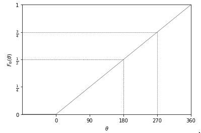
We can verify this result using simulation. To estimate cumulative distribution functions, we take \(M\) simulated values \(\theta^{(m)}\) and then sort them in ascending order.
import numpy as np

M = 100  # Set the value of M

theta = np.zeros(M)  # Create an empty numpy array for theta

# Generate M uniform random numbers between 0 and 360 and store them in theta
theta = np.random.uniform(low=0, high=360, size=M)

theta_ascending = np.sort(theta)  # Sort theta in ascending order

prob = np.arange(1, M+1) / M  # Calculate the probabilities
The expression (1:M) denotes the sequence \(1, 2, \ldots, M\), so that
(1:M) / M denotes \(\frac{1}{M}, \frac{2}{M}, \ldots, \frac{M}{M}\).
The trick is to put the sorted random variable the \(x\)-axis and the
probability values on the \(y\) axis. Here’s a run with \(M = 1,000\)
simulated values.
Plot of the cumulative distribution function of a random variable \(\theta\) representing the result of a fair spin of a spinner from 0 to 360 degrees. As expected, it is a simple linear function because the underlying variable \(\theta\) has a uniform distribution.
import numpy as np
import pandas as pd
from plotnine import ggplot, aes, geom_line, scale_x_continuous, scale_y_continuous, xlab, ylab

M = 1000
theta = np.random.uniform(0, 360, size=M)
theta_asc = np.sort(theta)
prob = np.arange(1, M+1) / M

unif_cdf_df = pd.DataFrame({'theta': theta_asc, 'prob': prob})
unif_cdf_plot = (
    ggplot(unif_cdf_df, aes(x='theta', y='prob')) +
    geom_line() +
    scale_x_continuous(breaks=[0, 90, 180, 270, 360]) +
    scale_y_continuous(breaks=[0, 0.25, 0.5, 0.75, 1.0]) +
    xlab('$\\theta$') +
    ylab('$F_\\Theta(\\theta)$')
)
unif_cdf_plot
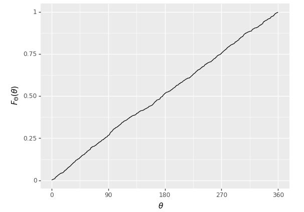
Even with \(M = 1,000\), this is pretty much indistinguishable from the one plotted analytically.
As with discrete parameters, the cumulative distribution function may be used to calculate interval probabilities, e.g.,^[With continuous variables, the interval probabilities are open below (\(180 < \Theta\)) and closed above (\(\Theta \leq 270\)), due to the definition of the cumulative distribution function as a closed upper bound (\(F_{\Theta}(\theta) = \mbox{Pr}[\Theta \leq \theta]\)).]
[\begin{array}{rcl} \mbox{Pr}[180 < \Theta \leq 270] & = & \mbox{Pr}[\Theta \leq 270] \ - \ \mbox{Pr}[\Theta \leq 180] \[2pt] & = & F_{\Theta}(270) - F_{\Theta}(180) \[2pt] & = & \frac{3}{4} - \frac{1}{2} \[2pt] & = & \frac{1}{4}. \end{array}]
The log odds transform
Now that we have seen how to generate uniform random numbers from 0 to 360, it is time to consider generating standard uniform variates from 0 to 1. Suppose \(\Theta\) is a random variable with a standard uniform distribution, i.e., \(\Theta \sim \mbox{uniform}(0, 1)\). Because probabilities are scaled from zero to one, we can think of \(\Theta\) as denoting a random probability.
Given a probability value \(\theta \in (0, 1)\), we can define its log odds by
[\mbox{logit}(\theta) = \log \frac{\theta}{1 - \theta}.]
This is just the natural logarithm of the odds, \(\frac{\theta}{1 - \theta}\). Now let
[\Phi = \mbox{logit}(\Theta)]
be the random variable representing the log odds. We say that \(\Phi\) is a transform of \(\Theta\), because its value is determined by the value of \(\Theta\).
Simulating transformed variables is straightforward.
import numpy as np

M = 1000
theta = np.random.uniform(0, 1, size=M)
alpha = np.log(theta / (1 - theta))

print(f'alpha = {alpha[:10]} ...')
alpha = [ 1.99678538 -1.77469355 -0.77809048  0.70232242  0.52317288 -2.15661683
 -1.72339989 -0.29737391 -3.47165039  0.2311787 ] ...
We can run this and see the first ten values,
import numpy as np

np.random.seed(1234)

M = 10000

def logit(x):
    return np.log(x / (1 - x))

theta = np.random.uniform(size=M)
alpha = logit(theta)

for m in range(10):
    print(f'{alpha[m]:.2f}', end=' ')

print('...')
-1.44 0.50 -0.25 1.30 1.27 -0.98 -0.96 1.40 3.13 1.95 ...
To understand the distribution of values of \(\Phi\), let’s look at histograms. First, we have the uniform draws of \(\Theta\), and then the transform to log odds \(\Phi = \mathrm{logit}(\Theta)\), Histogram of 10,000 simulated draws of \(\theta \sim \mbox{uniform}(0, 1)\).
import pandas as pd
from plotnine import ggplot, aes, geom_histogram, scale_x_continuous, scale_y_continuous, xlab
from plotnine.themes import theme_minimal

df_prob_unif = pd.DataFrame({'theta': theta})
unif_prob_plot = (
    ggplot(df_prob_unif, aes(x='theta')) +
    geom_histogram(binwidth=1/34, center=1/68, color='black',
                   fill='#ffffe6', size=0.25) +
    scale_x_continuous(breaks=[0, 0.25, 0.5, 0.75, 1]) +
    scale_y_continuous(limits=[0, 1300], breaks=[500, 1000]) +
    xlab('$\\theta$ ~ uniform(0, 1)') +
    theme_minimal()
)
unif_prob_plot
Histogram of 10,000 simulated draws of \(\theta \sim \mbox{uniform}(0, 1)\) transformed to the log odds scale by \(\Phi = \mbox{logit}(\theta).\)
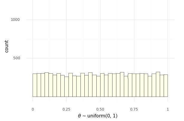
import pandas as pd
from plotnine import *
import numpy as np

np.random.seed(1234)

M = 10000
logit = lambda x: np.log(x / (1 - x))

theta = np.random.uniform(size=M)
alpha = logit(theta)

for m in range(10):
    print(f'{alpha[m]:.2f}', end=' ')
print('...')

df_prob_unif = pd.DataFrame({'theta': theta})
unif_prob_plot = (
    ggplot(df_prob_unif, aes(x='theta')) +
    geom_histogram(binwidth=1/34, center=1/68, color='black',
                   fill='#ffffe6', size=0.25) +
    scale_x_continuous(breaks=[0, 0.25, 0.5, 0.75, 1]) +
    scale_y_continuous(limits=[0, 1300], breaks=[500, 1000]) +
    xlab(r'$\Theta \sim \mathrm{uniform}(0, 1)$') +
    ggtitle('Probability density of uniform distribution') +
    theme_tufte()
)
unif_prob_plot

df_log_odds = pd.DataFrame({'alpha': alpha})
log_odds_plot = (
    ggplot(df_log_odds, aes(x='alpha')) +
    geom_histogram(binwidth=0.5, color='black', fill='#ffffe6',
                   size=0.25) +
    scale_x_continuous(breaks=[-6, -4, -2, 0, 2, 4, 6]) +
    scale_y_continuous(limits=[0, 1300], breaks=[500, 1000]) +
    xlab(r'$\varphi = \mathrm{logit}(\Theta)$') +
    ggtitle('Probability density of log-odds') +
    theme_tufte()
)
log_odds_plot
-1.44 0.50 -0.25 1.30 1.27 -0.98 -0.96 1.40 3.13 1.95 ...
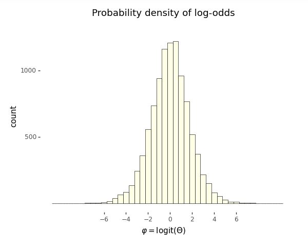
Even though the probability variable \(\Theta \sim \mbox{uniform}(0, 1)\) is uniform by construction, the log odds variable \(\Phi = \mbox{logit}(\Theta)\) is not distributed uniformly.
A further feature of the log odds plot is that the distribution of values is symmetric around zero. Zero on the log odds scale corresponds to 0.5 on the probability scale,^[Recall that the inverse log odds function is defined by \(\mbox{logit}^{-1}(u) = \frac{1}{1 + \exp(-u)}.\) This function is called the logistic sigmoid in engineering circles. Inverses satisfy for \(u \in \mathbb{R}\), \(\mbox{logit}(\mbox{logit}^{-1}(u)) = u\) and \(v \in (0, 1)\), \(\mbox{logit}^{-1}(\mbox{logit}(v)) = v.\)] i.e.,
[0 = \mbox{logit}(0.5),]
or equivalently,
[\mbox{logit}^{-1}(0) = 0.5.]
Unboundedness and symmetry around zero make log odds quite convenient statistically and will resurface in categorical regressions.
The third relevant feature of the log odds plot is that almost all of the values are within \(\pm 6\) of the origin. This is not surprising given that we took \(10,000\) draws and
[\mbox{logit}^{-1}(-6) = 0.0025]
and
[\mbox{logit}^{-1}(6) = 0.9975]
on the probability scale.
We can also do what we did for uniform distributions and plot the cumulative distribution based on simulation; we need merely insert the log-odds transform.
import numpy as np

M = 1000# define the value for M

theta = np.zeros(M)
for m in range(M):
    theta[m] = np.random.uniform(0, 360)

theta_ascending = np.sort(the
We again plot with \(M = 1,000\) simulated values.
Plot of the cumulative distribution function of a random variable \(\Phi = \mbox{logit}(\theta)\) representing the log odds transform of a uniformly distributed random variable \(\theta \sim \mbox{uniform}(0, 1)\). The curve it picks out is S-shaped. The asymptotes at 0 and 1 are indicated with dashed lines; the symmetries around 0 on the \(x\)-axis and 0.5 on the \(y\)-axis are picked out with dotted lines.
import numpy as np
import pandas as pd
import matplotlib.pyplot as plt
import seaborn as sns

def logit(u):
    return np.log(u / (1 - u))

M = 1000
phi = logit(np.random.uniform(size=M))
phi_asc = np.sort(phi)
prob = np.arange(1, M+1) / M

logistic_cdf_df = pd.DataFrame({'phi': phi_asc, 'prob': prob})
logistic_cdf_plot = sns.lineplot(data=logistic_cdf_df, x='phi', y='prob', axes=plt.gca())
logistic_cdf_plot.axhline(y=1, linestyle='--', linewidth=0.3, color='#333333')
logistic_cdf_plot.axhline(y=0, linestyle='--', linewidth=0.3, color='#333333')
logistic_cdf_plot.axvline(x=0, linestyle=':', linewidth=0.3, color='#333333')
logistic_cdf_plot.axhline(y=0.5, linestyle=':', linewidth=0.3, color='#333333')
logistic_cdf_plot.set(xlim=(-7, 7), xticks=[-6, -4, -2, 0, 2, 4, 6], yticks=[0, 0.25, 0.5, 0.75, 1.0])
logistic_cdf_plot.set(xlabel=r'$\phi$', ylabel=r'$F_{\Phi}(\phi)$')
sns.set_style('ticks')
plt.show()
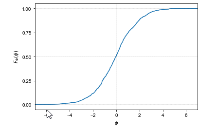
The result is an S-shaped function whose values lie between 0 and 1, with asymptotes at one as \(\theta\) approaches \(\infty\) and at zero as \(\theta\) approaches \(-\infty\). The argument of 0 has a value of 0.5.
The cumulative distribution function of this distribution is well known and has a closed analytic form based on the inverse of the log odds transform,
[F_{\Theta}(\theta)
\ =
\mathrm{logit}^{-1}(\theta)
\ =
\frac{1}{1 + \exp(-\theta)}.]
The inverse log odds function is itself known as the logistic sigmoid function.^[A name presumably derived from its shape and the propensity of mathematicians, like doctors, to prefer Greek terminology—the Greek letter “\(\sigma\)” (sigma) corresponds to the Roman letter “S”.]
Expectation and variance of continuous random variables
Just as with discrete random variables, the expectation of a continuous random variable \(Y\) is defined as a weighted average of its values. Only this time, the weights are defined by the probability density function rather than by the probability mass function. Because \(Y\) takes on continuous values, we’ll need calculus to compute the weighted average.
[\mathbb{E}[Y] = \int_{-\infty}^{\infty} y \times p_Y(y) \, \mathrm{d}y.]
Integrals of this general form should be read as a weighted average. It averages the value of \(y\) with weights equal to the density \(p_Y(y)\) of \(y\).^[Sometimes physicists will rearrange integral notation to reflect this and write \(\mathbb{E}[f(y)] = \int \mathrm{d}y \ p_Y(y) \times f(y)\) or even \(\mathbb{E}[f(y)] = \int p_Y(\mathrm{d}y) \times f(y).\)]
Variances are calculated just as they were for discrete variables, as
[\mbox{var}[Y]
\ =
\mathbb{E}\left[
\left(Y - \mathbb{E}[Y]\right)
\right].]
Let’s check this with some simulation by estimating the mean and variance of our running example. Suppose we have a a random variable \(\Phi = \mbox{logit}(\Theta)\), where \(\Theta \sim \mbox{uniform}(0, 1)\). We can estimate the expectation and variance of \(\Phi\) by simulating and calculating means and variances of the simulated values,
import numpy as np

np.random.seed(1234)

M = 1000
phi = np.zeros(M)

for m in range(M):
    phi[m] = logit(np.random.uniform())

E_Phi = np.sum(phi) / M
var_Phi = np.sum((phi - E_Phi)**2) / M

print(f"Estimated E[Phi] = {E_Phi}; var[Phi] = {var_Phi}; sd[Phi] = {np.sqrt(var_Phi)}")
Estimated E[Phi] = 0.05805343885611037; var[Phi] = 3.609094985913; sd[Phi] = 1.8997618234697211
Let’s run that for \(M = 1,000,000\) and see what we get.
import numpy as np

M = int(1e6)
phi = np.random.logistic(size=M)

E_Phi = np.sum(phi) / M
var_Phi = np.sum((phi - E_Phi)**2) / M

print(f"Estimated E[Phi] = {E_Phi:.2f}; var[Phi] = {var_Phi:.2f}; sd[Phi] = {np.sqrt(var_Phi):.2f}")
Estimated E[Phi] = -0.00; var[Phi] = 3.30; sd[Phi] = 1.82
The true value of the expectation \(\mathbb{E}[Y]\) is zero, and the true value of the variance is \(\frac{\pi^2}{3} \approx 3.29\).^[The true mean and variance for the logistic distribution can be calculated analytically. See the final section on this chapter for the analytic derivativation of the probability density function. The density must be integrated to analytically calculate the mean and variance, though the result for the mean also arises from symmetry.]
From histograms to densities
There is no equivalent of a probability mass function for continuous random variables. Instead, there is a probability density function, which in simulation terms may usefully be thought of as a limit of a histogram as the number of draws increases and the width of bins shrinks. Letting the number of simulations grow from \(10\) to \(1,000,000\), we see the limiting behavior of the histograms.
Histograms of \(M\) simulated draws of \(\theta \sim \mbox{uniform}(0, 1)\) transformed to the log odds scale by \(\Phi = \mbox{logit}(\theta).\) The limiting behavior is shown in the bell-shaped curve in the lower right based on \(1,000,000\) draws.
import numpy as np
import pandas as pd
import matplotlib.pyplot as plt
import seaborn as sns

np.random.seed(1234)

df_log_odds_growth = pd.DataFrame()
for log10M in range(1, 7):
    M = 10**log10M
    alpha = np.random.logistic(size=M)
    df = pd.DataFrame({'alpha': alpha, 'M': [f'M = {M}']*M})
    df_log_odds_growth = pd.concat([df_log_odds_growth, df], ignore_index=True)

# Define the grid
grid = sns.FacetGrid(df_log_odds_growth, col='M', col_wrap=3)

# Plot the histogram for each group
grid.map(
    sns.histplot,
    'alpha',
    element='step',
    stat='density',
    common_norm=False,
    bins=75,
    palette='colorblind'
)

# Set the axis labels and limits
grid.set(
    xlim=(-8.5, 8.5),
    xticks=[-5, 0, 5],
    xlabel=r'$\Phi = \mathrm{logit}(\Theta)$',
    ylabel='proportion of draws'
)

# Show the plot
plt.show()
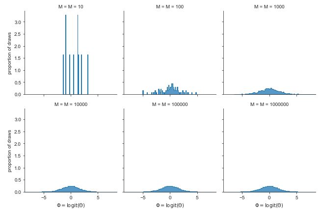
In a histogram, a bin’s height is proportional to the number of simulations that landed in that bin. Because each bin is the same width, a bin’s area (given by its width time its height) must also be proportional to the number of simulations that landed in that bin.
With simulation, the estimate of a probability landing in a bin is just the proportion of simulate values that land in the bin. Thus we can think of the area of a histogram’s bar as an estimate of the probability a value will fall in that bin.
Because the bins are exclusive (a number can’t fall in two bins), the probability of landing in either of two bins is proportional to the sum of their areas. This notion extends to intervals, where the estimated probability of the random variable falling between -2 and 2 is just the proportion of area between those two values in the histogram of simulations. Similarly, we can take a simulation-based estimate of \(\mbox{Pr}[\Theta \leq \theta]\) for any \(\theta\) as the proportion of simulated values that are less than or equal to \(\theta\). This is just the area to the left of the \(\theta\).
As the number of draws \(M\) increases, the estimated bin probabilities become closer and closer to the true values. Now we are going to look at the limiting continuous behavior. Put a point in the middle of the top of each histogram bar and connect them with lines. With a finite number of bins, that makes a jagged pointwise linear function. As the number of bins increases and the number of draws per bin increases, the function gets smoother and smoother. In the limit as \(M \rightarrow \infty\), it approaches a smooth function. That smooth function is called the probability density function of the random variable. Let’s see what that limiting function looks like with \(M = 1,000,000\) draws.
Histogram of \(M = 1,000,000\) simulations of \(\theta \sim \mbox{uniform}(0,1)\) transformed to \(\Phi = \mbox{logit}(\theta)\). The black line connects the tops of the histogram bins. In the limit, as the number of draws and bins approach infinity, the connecting line approaches the probability density function for the variable being simulated.
import numpy as np
import pandas as pd
import matplotlib.pyplot as plt
import seaborn as sns
from scipy.stats import logistic

np.random.seed(1234)

M = int(1e6)
alpha = logistic.rvs(size=M)
density_limit_df = pd.DataFrame({'alpha': alpha})

density_limit_plot = sns.histplot(
    data=density_limit_df,
    x='alpha',
    stat='density',
    bins=75,
    color='blue',
    alpha=0.5
)
density_limit_plot.set(
    xlim=(-9, 9),
    xticks=[-6, -4, -2, 0, 2, 4, 6],
    xlabel=r'$\Phi = \mathrm{logit}(\Theta)$',
    ylabel='proportion of draws'
)
density_limit_plot.plot(
    np.linspace(-9, 9, num=1000),
    logistic.pdf(np.linspace(-9, 9, num=1000), loc=0, scale=1),
    color='red',
    linewidth=0.5
)
sns.set_style("ticks", {"xtick.major.size": 2, "ytick.major.size": 2})
sns.despine(offset=5)
plt.show()
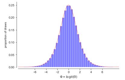
A detour through calculus
We have seen that the probability of a variable falling in an interval is estimated by proportion of the overall histogram area falls in the interval—that is, the sum of the histogram areas in the interval. What we want to do is let the number of bins and number of draws continue to increase to get ever better approximations. When we let the number of bins increase toward infinity, we have a familiar limit from integral calculus.
If \(p_Y(y)\) is the continuous density function we get as the limit of the histogram, then the probability that \(Y\) falls between \(a\) and \(b\) is given by the proportion of area between \(a\) and \(b\) in the function \(p_Y(y)\). This is the key insight for understanding density functions and continuous random variables. For bounded intervals, we have
[\mbox{Pr}[a \leq Y \leq b]
\ \propto
\int^b_a \ p_Y(y) \, \mathrm{d}y.]
To make our lives easier and avoid writing the proportional-to symbol (\(\propto\)) everywhere, we will make the conventional assumption that our density functions like \(p_Y\) are normalized. This means that the total area under their curve is one,
[\int_{-\infty}^{\infty} p_Y(y) \, \mathrm{d}y \ = \ 1.]
Because they are based on the limits of histograms, which are counts, we will also meet the standard requirement placed on density functions that they be positive, so that for all \(y \in \mathbb{R}\),
[p_Y(y) \geq 0.]
With these assumptions in place, we now define interval probabilities using definite integration over density functions,
[\mbox{Pr}[a \leq Y \leq b]
\ =
\int^b_a \ p_Y(y) \, \mathrm{d}y.]
For simple upper bounds, we just integrate from negative infinity,
[\mbox{Pr}[Y \leq b]
\ =
\int_{-\infty}^b \ p_Y(y) \, \mathrm{d}y.]
This reveals the relation between the cumulative distribution function \(F_Y) = \mbox{Pr}[Y \leq b]\) and the probability density function \(p_Y\)
[F_Y(b) \ = \ \int_{-\infty}^b \ p_Y(y) \, \mathrm{d}y.]
Working the other way around, it reveals that the probability density function is just the derivative of the cumulative distribution function,
| [p_Y(b) = \frac{\mathrm{d}}{\mathrm{d}y} F_Y(y) \Bigg | _{y = b}.] |
Thus the units of a probability density function are change in cumulative probability, not probability. Density functions must be integrated to get back to units of probability.
The uniform density function
We’ve already seen the histograms for variables \(\Theta \sim \mbox{uniform}(0, 1)\) distributed uniformly from zero to one. With an increasing numbers of draws, the histograms flatten out. With more draws the histograms will level out even more until the density becomes a straight line. This means that the probability density function of a uniformly distributed random variable is constant.^[Another way to reach the same conclusion is by calculus. We worked out from first principles that the cumulative distribution function is linear if uniformity means equal probability of landing in any interval of the same size. The derivative of a linear function is constant, so the density for a uniform distribution must be constant.] That is, if \(\Theta \sim \mbox{uniform}(a, b)\), then \(p_{\Theta}(\theta) = c\) for some constant \(c\). Let’s see what that looks like so the solution for \(c\) becomes evident.
import pandas as pd
import matplotlib.pyplot as plt
import seaborn as sns

uniform_pdf_df = pd.DataFrame({'y': [0, 1], 'p_y': [1, 1]})
sns.set(rc={'figure.figsize':(4,4)})
uniform_pdf_plot = sns.lineplot(data=uniform_pdf_df, x='y', y='p_y', marker='o', color='#333333')
uniform_pdf_plot.set(xticks=[0, 1], xticklabels=['a', 'b'], yticks=[0, 1], yticklabels=['0', 'c'], xlim=(-0.1, 1.1), ylim=(-0.1, 1.1), xlabel=r'$\theta$', ylabel=r'$p_{\Theta}(\theta|a,b)$')
uniform_pdf_plot.axhline(y=1, xmin=-0.1, xmax=0, linestyle='dotted')
uniform_pdf_plot.axhline(y=1, xmin=1, xmax=1.1, linestyle='dotted')
uniform_pdf_plot.axvline(x=0, ymin=0, ymax=1, linestyle='dotted')
uniform_pdf_plot.axvline(x=1, ymin=0, ymax=1, linestyle='dotted')
uniform_pdf_plot.text(-0.2, -0.1, '0')
uniform_pdf_plot.text(1.05, -0.1, '1')
plt.show()
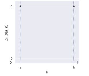
The plot shows the area from \(a\) to \(b\) under \(c\) to be \((b - a) \times c\). Given that we require the area to be one, that is, \((b - a) \times c = 1\), we can work out \(c\) by dividing both sides by \(b - a\),
[c = \frac{\displaystyle{1}}{\displaystyle b - a}.]
Putting this into density notation, if \(\Theta \sim \mbox{uniform}(a, b)\), then
[p_{\Theta}(\theta) = \mbox{uniform}(\theta \mid a, b),]
where we have now worked out that
[\mbox{uniform}(\theta \mid a, b) = \frac{1}{b - a}.]
That is, the density does not depend on \(y\)—it is constant and the same for every possible value of \(\theta\).^[For convenience, we can assume the impossible values of \(\theta\) have density zero.]
Back to simulation
The traditional bottleneck to performing statistics beyond the data collection was wrangling integral calculus to provide analytic results or approximations for a given applied problem. Today, very general numerical solvers absolve us of the heavy lifting of calculus and replace it with wrangling computer code for simulations. This lets us solve much harder problems directly.
Let’s actually solve the integral we mentioned in the last section, namely the probability that a log odds variable will land between -2 and 2.
import numpy as np

success = 0
M = 1000 # replace with desired number of iterations
for m in range(1, M+1):
    Phi = np.random.uniform(0, 1)
    Phi = np.log(Phi / (1 - Phi))
    if -2 < Phi < 2:
        success += 1

print('Pr[-2 < Phi < 2] =', success / M)
Pr[-2 < Phi < 2] = 0.759
Let’s run that for \(M = 100,000\) simulation draws and see what we get,
import numpy as np

np.random.seed(1234)
M = 100000
Phi = np.log(np.random.uniform(0, 1, M) / (1 - np.random.uniform(0, 1, M)))
success = 0
for m in range(M):
    if -2 < Phi[m] < 2:
        success += 1

print('Pr[-2 < Phi < 2] =', '{:.2f}'.format(success / M))
Pr[-2 < Phi < 2] = 0.87
What is perhaps more remarkable than not requiring calculus is that we don’t even require the formula for the density function \(p_{\Phi}\)—we only need to be able to simulate random instantiations of the random variable in question.
Laws of probability for densities
Whether a random variable \(Y\) is continuous or discrete, its cumulative distribution function \(F_Y\) is defined by
[F_Y(y) = \mbox{Pr}[Y \leq y].]
Using simulation, if \(Y\) is a continuous random variable, its probability density function \(p_Y\) is the limit of the histogram of simulation draws. Using calculus, the density \(p_Y\) of a continuous random variable \(Y\) is defined as the derivative of the cumulative distribution function \(F_Y\),^[Differential notation avoids the fiddly notation arising from bound variables, e.g., \(p_Y(y) \ = \ \frac{\mathrm{d}}{\mathrm{d}y} F_Y(y).\) With multivariate functions, the derivative operator is replaced with the gradient operator \(\nabla.\)]
[p_Y = \mathrm{d} F_Y.]
Joint cumulative distribution functions for a pair of continuous random variables \(X, Y\) are defined as expected,
[F_{X, Y}(x, y) = \mbox{Pr}[X \leq x \ \mbox{and} \ Y \leq y],]
and may be easily extended to more variables. With simulation, cumulative distribution functions may be recreated by sorting the simulated values and normalizing.
Joint densities for a pair \(X, Y\) of continuous random variables are defined by differentiating the joint cumulative distribution twice,^[With bound variables, \(p_{X, Y}(x, y) = \frac{\partial^2}{\partial x \partial y} F_{X, Y}(x, y).\)]
[p_{X, Y} = \mathrm{\partial^2} F_{X, Y}.]
Marginal densities \(p_X\) may now be defined in terms of the joint density \(p_{X, Y}\) by integration,^[If we had a convenient integral operator, we could avoid the bound variable fiddling. As written, in the traditional style, it is muddied that the integral just averages over \(y\) treating \(x\) as a variable bound by the function definition notation.]
[p_X(x) = \int_{-\infty}^{\infty} p_{X, Y}(x, y) \, \mathrm{d}y.]
With simulation, if we can simulate \(x^{(m)}, y^{(m)}\) jointly, then we can simulate \(x^{(m)}\) by simply dropping \(y^{(m)}\).
If we can simulate from \(Y\), we can compute \(p_X(x)\) for a given value of \(x\) by averaging,
[p_X(x)
\ \approx
\frac{1}{M} \sum_{m \in 1:M} p_{X,Y}(x, y^{(m)}).]
Conditional densities \(p_{X \mid Y}\) are defined by dividing the joint density \(p_{X, Y}\) by the marginal density \(p_{X}\),
[p_{X \mid Y}(x \mid y)
\ =
\frac{\displaystyle p_{X, Y}(x, y)}
{p_Y(y)}.]
Conditional densities \(p_{X \mid Y}(x \mid y)\) may be handled by simulation for specific values of \(y\).
Equivalently, we can see this as a definition of the joint density in terms of the conditional and marginal,
[p_{X, Y}(x, y)
\ =
p_{X \mid Y}(x \mid y) \times p_Y(y).]
With simulation, this is often the strategy to generate simulations from the joint distribution—first simulate from \(Y\), then simulate \(X\) given \(Y\).
A convenient form of marginalization uses this definition,
[p_X(x) = \int_{-\infty}^{\infty} p_{X \mid Y}(x, y) \times p_Y(y) \, \mathrm{d} y.]
Continuous random variables \(X\) and \(Y\) are independent if their densities factor, so that for all \(x, y\),
[p_{X, Y}(x, y)
\ =
p_X(x) \times p_Y(y),]
or equivalently,
[p_{X \mid Y}(x \mid y)
\ =
p_X(x).]
Expectations for continuous random variables are defined using integration to calculate the average of \(y\) weighted by the density \(p_Y(y)\),
[\mathbb{E}[Y]
\ =
\int_{-\infty}^{\infty} y \times p_Y(y) \, \mathrm{d}y.]
In moving from discrete to continuous variables, we have merely switched the definition from summation to integration. Luckily, calculation by simulation need not change—we will still be calculating expectations by averaging over simulated values. If we can simulate \(y^{(m)}\) according to \(p_Y(y)\) for \(m \in 1:M\), our simulation-based estimate is
[\mathbb{E}[f(y)]
\ \approx
\frac{1}{M} \sum_{m = 1}^M
f ! \left( y^{(m)} \right).]
This estimate becomes exact as \(M \rightarrow \infty\).
Variances are defined in terms of expectation, just as before,
[\mbox{var}[Y]
\ =
\mathbb{E}\left[
\left(
Y - \mathbb{E}[Y]
\right)^2
\right]
\ =
\mathbb{E}[Y^2]
- \left( \mathbb{E}[Y] \right)^2.]
Variances can be estimated through simulation like any other expectation.^[The sample variance computed by standard software divides by \(M - 1\) to correct for the bias introduced by using the sample mean to estimate variance. The maximum likelihood estimate resulting from dividing by \(M\) is biased to underestimate variance with finite samples; asymptotically, it provides the correct result, because the \(\frac{M}{M-1}\) correction factor approaches one as \(M\) increases.]
Jacobians and changes of variables
When we moved from a random variable \(\Theta \sim \mbox{uniform}(0, 1)\) to a variable \(\Phi = \mbox{logit}(\Theta)\), we made a class change of variables. That means we can use calculus to compute the probability density function. But let’s do it in full generality.
We’ll start by assuming we have a random variable \(X\) with a known density function \(p_X(x)\). Assume further we have a smooth and invertible function \(f\) and define a new random variable \(Y = f(X)\). The density of \(Y\) is then given by the rather daunting formula
[p_Y(y)
\ =
p_X(f^{-1}(y))
\, \times \,
\left|
\,
\frac{\mathrm{d}}
{\mathrm{d}u}
f^{-1}(u) \Big|_{u = y}
\,
\right|.]
We’re going to work through this in pieces using our running example. To keep the puzzle pieces straight, let \(X = \Theta \sim \mbox{uniform}(0, 1)\) be our uniform probability variable and \(Y = \Phi = \mbox{logit}(\Theta)\) be the transformed variable on the log odds scale. Our goal is to calculate the density of \(\Phi\) given that we know the density of \(\Theta\) and the transform from \(\Theta\) to \(\Phi\). We begin by noting that
[\mbox{logit}^{-1}(y) = \frac{1}{1 + \exp(-y)}.]
So to evaluate \(p_{\Phi}(\phi)\), we first need to evaluate \(p_{\Theta}(\mbox{logit}^{-1}(\phi))\). We know this term will evaluate to 1, because \(p_{\Theta}(\theta) = 1\) for every \(\theta\). So clearly just inverting and plugging in isn’t enough.
We also need to account for the change in variables from \(\Theta\) to \(\Phi\). This is where the Jacobian term comes into the equation—that’s everything past the \(\times\) sign. The Jacobian is the absolute value of the derivative of the inverse transform evaluated at the value in question. For our running example, we can work out through the chain rule that
[\frac{\mathrm{d}}{\mathrm{d} u}
\mbox{logit}^{-1}(u)
\ =
\mbox{logit}^{-1}(u)
\times \left(1 - \mbox{logit}^{-1}(u)\right).]
So if we plug in \(u = \phi\) here, and put all the pieces back together, we get
[p_{\Phi}(\phi)
\ =
\mbox{logit}^{-1}(\phi)
\times
\left( 1 - \mbox{logit}^{-1}(\phi) \right).]
This distribution is known as the standard logistic distribution,
[\mbox{logistic}(\phi \mid 0, 1)
\ =
\mbox{logit}^{-1}(\phi)
\times
\left( 1 - \mbox{logit}^{-1}(\phi) \right).]
Thus after all the dust has settled, we know that if \(\Theta \sim \mbox{uniform}(0, 1)\) and \(\Phi = \mbox{logit}(\Theta)\), then \(\Phi \sim \mbox{logistic}(0, 1)\).^[The meaning of the parameters 0 and 1 will be explained in the next section.]
Exponential distributions
We have already seen that if we take a uniformly distributed variable, \(U \sim \textrm{uniform}(0, 1),\) and log-odds transform it to \(V = \textrm{logit}(U),\) the resulting variable has a standard logistic distribution, \(V \sim \textrm{logistic}(0, 1).\)
In this section, we consider a negative log transform, \(Y = -\log U,\) We know that if \(U \in (0, 1)\), then \(\log U \in (-\infty, 0)\), and hence \(Y = -\log U \in (0, \infty).\)
Let’s plot a histogram of simulated values of \(Y\) to see what its density looks like. The simulation is trivial.
import numpy as np

u = np.random.uniform(0, 1)
y = -np.log(u)
We’ll generate \(M = 10^6\) draws and calculate some summary statistics.
import numpy as np

y = -np.log(np.random.uniform(0, 1, 1000))
print("mean(y) = {:.2f}".format(np.mean(y)))
print("sd(y) = {:.2f}".format(np.std(y)))
print("central 95 pct interval = ({:.2f}, {:.2f})".format(np.quantile(y, 0.025), np.quantile(y, 0.975)))
print("min = {:.2f};  max = {:.2f}".format(np.min(y), np.max(y)))
mean(y) = 1.04
sd(y) = 0.98
central 95 pct interval = (0.03, 3.65)
min = 0.00;  max = 5.97
It’s clear that the variable has a mean and standard deviation of one, but is highly right skewed.
Histogram of \(M = 10^6\) draws from \(U \sim \textrm{uniform}(0, 1)\) transformed to \(Y = -\log U.\) The mean and standard deviation are 1, but the distribution is highly right skewed.
import numpy as np
import pandas as pd
import matplotlib.pyplot as plt
import seaborn as sns

y = -np.log(np.random.uniform(0, 1, 1000000))
exp_df = pd.DataFrame({'y': y})
exp_hist_plot = sns.histplot(exp_df, x='y', color='#ffffe6', edgecolor='black',
                             bins=100, stat='density')
exp_hist_plot.set(xlabel='y', ylabel='density')
plt.show()
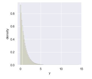
While the histogram plot lets us visualize the density, we can also derive the density \(p_Y\) from the uniform density \(p_U\) given the transform
[Y \ = \ f(U) \ = \ -\log U.]
First, we calculate the inverse transform,
[\begin{array}{rcl} Y & = & -\log U \[3pt] -Y & = & \log U \[3pt] \exp(-Y) & = & U \end{array}]
so that
[f^{-1}(Y) = \exp(-U).]
We’ll need the derivative of this inverse for the Jacobian,^[We need to employ the chain rule here,
[\frac{\textrm{d}}{\textrm{d}x} a(b(x))
\ =
\left( \frac{\textrm{d}}{\textrm{d}u} a(u) \Bigg|_u = b(x) \right)
\cdot
\left( \frac{\textrm{d}}{\textrm{d}{x}} b(x) \right),]
with \(a(u) = \exp(u)\) and \(b(x) = -x.\)
[\begin{array}{rcl} \frac{\textrm{d}}{\textrm{d}y} f^{-1}(y) & = & \frac{\textrm{d}}{\textrm{d}y} \exp(-y) \[4pt] & = & -\exp(-y). \end{array}]
We can now derive the density of \(Y = f(U) = -\log U\), where \(U \sim \textrm{uniform}(0, 1),\)
[\begin{array}{rcl} p_Y(y) & = & p_U(f^{-1}(y)) \cdot \left| \frac{\textrm{d}}{\textrm{d}y} \exp(-y) \right| \[8pt] & = & \textrm{uniform}(f^{-1}(y) \mid 0, 1) \cdot \left| -\exp(-y) \right| \[8pt] & = & \exp(-y). \end{array}]
The result, as simple as it looks, is a properly normalized density.^[Given the derivative \(\frac{\textrm{d}}{\textrm{d}y} -\exp(-y) \ = \ \exp(-y),\) the basic rule for computing definite integrals,
[\begin{array}{rcl}
\int_a^b f(x) \, \textrm{d}x
& = &
\int f(x) \, \textrm{d}x \, \Big|{x = b}
\ -
\int f(x) \, \textrm{d}x \, \Big|{x = a}
\[6pt]
& = & -\exp(-x)\Big|{x = b} - -\exp(-x)\Big|{x = a}
\[6pt]
& = & -\exp(-b) + \exp(-a).
\end{array}]]
Plugging in \(a = 0\) and \(b = \infty\) (the latter is really taking a limit), gives us \(-\exp(-\infty) + \exp(-0) = 0 + 1 = 1.\)
This distribution is popular enough to get its own name, the exponential distribution, the standard version of which is conventionally defined by
[\textrm{exponential}(y \mid 1) = \exp(-y).]
As for other distributions, we will write \(Y \sim \textrm{exponential}(1)\) if \(p_Y(y) = \textrm{exponential}(y) = \exp(-y).\)
We will generalize the standard exponential by allowing it to be scaled. Unlike the normal distribution, which scales a standard normal by multiplying it by a scale parameter, it is conventional to divide a standard exponential variate by a rate parameter to get a general exponential variate. Suppose \(V \sim \textrm{exponential}(1)\) and we define a new variable \(Y = V / \lambda\) for some rate \(\lambda > 0.\) [A rate parameter divides a variable in contrast to a rate parameter, which multiplies a parameter.] This gives us a general exponential variate, \(Y \sim \textrm{exponential}(\lambda).\)
To define the general exponential density, we just apply the Jacobian formula again, keeping in mind that our transform is
[h(V) = V / \lambda,]
which has an inverse
[h^{-1}(Y) = \lambda \cdot Y.]
Plugging this into the formula for a change of variables, we get
[\begin{array}{rcl} p_Y(y) & = & p_V\left(h^{-1}(y)\right) \cdot \left| \frac{\textrm{d}}{\textrm{d}y} h^{-1}(y) \right| \[8pt] & = & p_V(\lambda \cdot y) \cdot \left| \frac{\textrm{d}}{\textrm{d}y} \lambda \cdot y \right| \[8pt] & = & \exp(-\lambda \cdot y) \cdot \lambda. \end{array}]
This gives us the final form of the exponential distribution,
[\textrm{exponential}(y \mid \lambda)
\ =
\lambda \cdot \exp(-\lambda \cdot y).]
By construction, we know that if the standard distribution has a mean of 1, then the transformed version has a mean of \(1 / \lambda.\) Similarly, the transformed version also has a standard deviation of \(1 / \lambda\).^[The inverse cumulative distribution function for the standard exponential is just the function \(-\log u\) used to construct the variable. It is thus simple symbolically to derive the cumulative distribution function and the generalized version with a non-unit rate.]
Key Points
Statistical Inference and Inverse Problems
Overview
Teaching: min
Exercises: minQuestions
Objectives
Statistical Inference and Inverse Problems
Deductive inference works from facts toward conclusions deterministically. For example, if I tell you that all men are mortal and that Socrates is a man, you can deductively conclude that Socrates is mortal. Inductive inference, on the other hand, is a bit more slippery to define, as it works from observations back to facts. That is, if we think of the facts as governing or generating the observations, then induction is a kind of inverse inference. Statistical inference is a kind of inductive inference that is specifically formulated as an inverse problem.
Laplace’s birth ratio model
The roots of statistical inference lie not in games of chance, but in the realm of public health. Pierre-Simon Laplace was investigating the rate of child births by sex in France in an attempt to predict future population sizes.^[Pierre-Simon Laplace. 1812. Essai philosophique sur les probabilités. H. Remy. p. lvi of the Introduction. Annotated English translation of the 1825 Fifth Edition: Andrew I. Dale, 1995. Philosophical Essay on Probabilities. Springer-Verlag.] Laplace reports the following number of live births, gathered from thirty departments of France between 1800 and 1802 was as follows.
[\begin{array}{r|r}
\mbox{sex} & \mbox{live births}
\ \hline
\mbox{male} & 110\,312
\mbox{female} & 105\,287
\end{array}]
Laplace assumed each birth is independent and each has probability \(\Theta \in [0, 1]\) of being a boy. Letting \(Y\) be the number of male births and \(N\) be the total number of births, Laplace assumed the model
[Y \sim \mbox{binomial}(N, \Theta).]
In other words, his data-generating distribution had the probability mass function^[The constant \(N\) that appears in the full binomial notation is suppressed in the density notation \(p_{Y \mid \Theta}\)—it is common to suppress constants in the notation to make the relationship between the modeled data \(Y\) and parameters \(\Theta\) easier to scan.]
[p_{Y \mid \Theta}(y \mid \theta)
\ =
\mbox{binomial}(y \mid N, \theta).]
Because it employs a binomial distribution, this model assumes that the sex of each baby is independent, with probability \(\theta\) of being a boy. This may or may not be a good approximation to reality. Part of our job is going to be to check the assumptions like this built into our models.
We know how to generate \(Y\) given values for the parameter \(\Theta\), but we are now faced with the inverse problem of drawing inferences about \(\Theta\) based on observations about \(Y\).
What is a model?
We say that this simple formula is a model in the sense that it is not the actual birth process, but rather a mathematical construct meant to reflect properties of the birth process. In this sense, it’s like Isaac Newton’s model of the planetary motions using differential equations.^[Isaac Newton. 1687. Philosophiae Naturalis Principia Mathematica. Translated as I. Bernard Cohen and Anne Whitman. 1999. The Principia: Mathematical Principles of Natural Philosophy. University of California Press.] The equations are not the planets, just descriptions of how they move in response to gravitational and other forces.
Models like Newton’s allow us to predict certain things, such as the motion of the planets, the tides, and balls dropped from towers. But they typically only approximate the full process being modeled in some way. Even Newton’s model, which is fabulously accurate at predictions at observable scales, is only an approximation to the finer-grained models of motion and gravity introduced by Albert Einstein.^[Einstein, Albert. 1907. Über das Relativitätsprinzip und die aus demselben gezogenen Folgerungen. (English translation: On the relativity principle and the conclusions drawn from it.) Jahrbuch der Radioaktivität und Elektronik 4:411–462.] which itself was only a special case of the more general theory of relativity.^[Einstein, Albert. 1916. The foundation of the general theory of relativity. Annalen Phys. 14:769–822.] Each successive model is better than the last in that it’s better at prediction, more general, or more elegant—science does not progress based on a single criterion for improving models.
The reproductive process is complex, and many factors may impinge on the sex of a baby being born. Part of our job as scientists is to check the assumptions of our models and refine them as necessary. This needs to be done relative to the goal of the model. If the goal of this simple reproductive model is only to predict the prevalence of male births at a national scale, then a simple, direct prevalence model with a single parameter like the one we have introduced may be sufficient.
To conclude, when we say “model”, all we have in mind is some mathematical construct taken to represent some aspect of reality. Whether a model is useful is a pragmatic question which must be judged relative to its intended application.
What is a random variable?
As in all statistical modeling, Laplace treated the observed number of male births \(Y\) as a random variable. This assumes a form of counterfactual reasoning whereby we assume the world might have been some other way than it actually turned out to be.
As in most statistical models, Laplace treated \(N\) as a constant. In many cases, the denominator of binary events is not itself a constant, but is itself a random variable determined by factors of the environment. For instance, the number of attempts an athlete on a sports team get depends on the ability of that athlete and the number of reviews a movie receives depends on its popularity.
As originally formulated by Thomas Bayes,^[Bayes, T., 1763. LII. An essay towards solving a problem in the doctrine of chances. By the late Rev. Mr. Bayes, FRS communicated by Mr. Price, in a letter to John Canton, AMFRS. Philosophical Transactions of the Royal Society, pp. 370–418.] Laplace also treated \(\Theta\) as a random variable. That is, Laplace wanted to infer, based on observation and measurement, that the probability that \(\Theta\)’s value was in a certain range. Specifically, Laplace was curious about the question of whether the male birth rate is higher, which can be expressed in probabilistic terms by the event probability \(\mbox{Pr}[\Theta > 0.5]\).
Laplace’s inverse problem
Given a total of \(N\) births, we have introduced random variables for
- the observed data of \(Y\) male births, and
- the probability \(\Theta\) that a live birth will result in a boy.
We also have the actual observed number of male births, \(y\). That is, we know the value of the random variable \(Y\). Given our observed data, we can ask two obvious questions, namely
- What is the probability of a boy being born?
- Is it more likely that a boy is born than a girl?
Given that \(\Theta\) is the male birth rate, the first question is asking about the value of \(\Theta\). To provide a probabilistic answer, we want to look at the distribution of \(\Theta\) given that we observe the actual data \(Y = y\), which has the density \(p_{\Theta \mid Y}(\theta \mid y)\). We can summarize this distribution probabilistically using intervals, for instance by reporting the central 95% interval probability,
[\mbox{Pr}\left[ 0.025 \leq \Theta \leq 0.975
\ \Big|
Y = y
\right].]
The second question, namely whether boys are more likely to be born, is true if \(\Theta > \frac{1}{2}\). The probability of this event is
[\mbox{Pr}\left[ \Theta > \frac{1}{2}
\ \Bigg|
Y = y
\right].]
If we can estimate this event probability, we can answer Laplace’s second question.^[The quality of the answer will be determined by the quality of the data and the quality of the model.]
Bayes’s rule to solve the inverse problem
The model we have is a generative model^[Also known as a forward model or a mechanistic model by scientists.]—it works from a parameter value \(\theta\) to the observed data \(y\) through a sampling distribution with probability function \(p_{Y \mid \Theta}(y \mid \theta).\) What we need to solve our inference problems is the posterior density \(p_{\Theta \mid Y}(\theta \mid y)\). Bayes realized that the posterior could be defined in terms of the sampling distribution as
[\begin{array}{rcl} p_{\Theta \mid Y}(\theta \mid y) & = & \frac{\displaystyle p_{Y \mid \Theta}(y \mid \theta) \times p_{\Theta}(\theta)} {\displaystyle p_Y(y)} \[6pt] & \propto & p_{Y \mid \Theta}(y \mid \theta) \times p_{\Theta}(\theta). \end{array}]
All of our sampling algorithms will work with densities known only up to a proportion.
The prior distribution
This still leaves the not inconsequential matter of how to determine \(p_{\Theta}(\theta)\), the density of the so-called prior distribution of \(\Theta\). The prior distribution encapsulates what we know about the parameters \(\Theta\) before observing the actual data \(y\). This prior knowledge may be derived in many different ways.
- We may have prior knowledge from physical constraints. For example, if we are modeling the concentration of a molecule in a solution, the concentration must be positive.
- We may have prior knowledge of the basic scale of the answer from prior scientific knowledge. For example, if we are modeling human growth, we know that heights above two meters are rare and heights above three meters are unheard of.
- We may have prior knowledge from directly related prior experiments. For example, if we are doing a Phase II drug trial, we will have data from the Phase I trial, or we may have data from Europe if we are doing a trial in the United States.
- We may have experiments from indirectly related trials. For example, if we are modeling football player abilities, we have years and years of data from prior seasons. We know nobody is going to average 10 points a game—it’s just not done.
Because we are working probabilistically, our prior knowledge will itself be modeled with a probability distribution, say with density \(p_{\Theta}(\theta)\). The prior distribution may depend on parameters, which may be constants or may themselves be unknown. This may seem like an awfully strong imposition to have to express prior knowledge as a density. If we can express our knowledge well and sharply in a distribution, we will have an informative prior. Luckily, because we are only building approximate models of reality, the prior knowledge model does not need to be perfect. We usually err on the side of underpowering the prior a bit compared to what we really know, imposing only weakly informative priors, such as those that determine scales, but not exact boundaries of parameters.^[The notion of a truly uninformative prior is much trickier, because to be truly uninformative, a prior must be scale free.]
We will have a lot to say about prior knowledge later in the book, but for now we can follow Laplace in adopting a uniform prior for the rate of male births,
[\Theta \sim \mbox{uniform}(0, 1).]
In other words, we assume the prior density is given by
[p_{\Theta}(\theta) = \mbox{uniform}(\Theta \mid 0, 1).]
Here, the bounds zero and one, expressed as constant parameters of the uniform distribution, are logical constraints imposed by the fact that the random variable \(\Theta\) denotes a probability.
Other than the logical bounds, this uniform prior distribution is saying a value in the range 0.01 to 0.05 is as likely as one in 0.48 to 0.52. This is a very weak prior indeed compared to what we know about births. Nevertheless, it will suffice for this first analysis.
The proportional posterior
With a prior and likelihood,^[Remember, the likelihood is just the sampling distribution \(p_{Y \mid \Theta}(y \mid \theta)\) viewed as a function of \(\theta\) for fixed \(y\).] we have our full joint model in hand,
[p_{Y \mid \Theta}(y \mid N, \theta) \times p_{\Theta}(\theta)
\ =
\mbox{binomial}(y \mid N, \theta)
\times \mbox{uniform}(\theta \mid 0, 1).]
We have carried along the constant \(N\) so we don’t forget it, but it simply appears on the right of the conditioning bar on both sides of the equation.
The sampling distribution \(p(y \mid \theta)\) is considered as a density for \(y\) given a value of \(\theta\). If we instead fix \(y\) and view \(p(y \mid \theta)\) as a function of \(\theta\), it is called the likelihood function. As a function, the likelihood function is not itself a density. Nevertheless, it is crucial in posterior inference.
With Bayes’s rule, we know the posterior is proportional to the prior times the likelihood,
[\underbrace{p_{\Theta \mid Y}(\theta \mid y)}{\text{posterior}}
\ \propto
\underbrace{p{Y \mid \Theta}(y \mid \theta)}{\text{likelihood}}
\ \times
\underbrace{p{\Theta}(\theta)}_{\text{prior}}.]
Given the definitions of the relevant probability functions,^[ For reference, these are the likelihood \(\mbox{binomial}(y \mid N, \theta) \ \propto \ \theta^y \times (1 - \theta)^{N - y}\) and the prior \(\mbox{uniform}(\theta \mid 0, 1) \ = \ 1.\) ] we have
[\begin{array}{rcl} p_{\Theta \mid Y}(\theta \mid y, N) & \propto & \mbox{binomial}(y \mid N, \theta) \times \mbox{uniform}(\theta \mid 0, 1) \[4pt] & \propto & \theta^y \times (1 - \theta)^{N - y} \end{array}]
To summarize, we know the posterior \(p_{\Theta \mid Y}\) up to a proportion, but are still missing the normalizing constant so that it integrates to one.^[We return to the normalizer later when we discuss the beta distribution.]
Sampling from the posterior
Now that we have a formula for the posterior up to a proportion, we are in business for sampling from the posterior. All of the sampling algorithms in common use require the density only up to a proportion.
For now, we will simply assume a method exists to draw a sample \(\theta^{(1)}, \cdots, \theta^{(M)}\) where each \(\theta^{(m)}\) is drawn from the posterior \(p_{\Theta \mid y}(\theta \mid y)\) given the observed data \(y\).
When we do begin to employ general samplers, they are going to require specifications of our models that are exact enough to be programmed. Rather than relying on narrative explanation, we’ll use a pseudocode for models that can be easily translated for an assortment of posterior samplers.^[This specification is sufficient for coding a sampler in BUGS, Edward, emcee, Greta, JAGS, NIMBLE, PyMC, Pyro, or Stan.]
[\begin{array}{r|lr}
\mbox{Name} & \mbox{simple binomial}
\ \hline
\mbox{Data}
& N \in \mathbb{N}
& y_n \in { 0, 1 }
& \mbox{ } \hfill \mbox{for} \ n \in 1:N
\ \hline
\mbox{Parameters}
& \theta \in (0, 1)
\ \hline
\mbox{Prior}
& \theta \sim \mbox{uniform}(0, 1)
\ \hline
\mbox{Likelihood}
& y_n \sim \mbox{binomial}(N, \theta)
& \mbox{ } \hfill \mbox{for} \ n \in 1:N
\end{array}]
Simulating data
Rather than starting with Laplace’s data, which will present computational problems, we will start with some simulated data. We simulate data for a model by simulating the parameters from the prior, then simulating the data from the parameters. That is, we run the model in the forward direction from prior to parameters to data. This is usually how we construct the models in the first place, so this should be a natural step. In pseudocode, this is a two-liner.
from random import uniform, randint

theta = uniform(0, 1)
y = randint(0, N)  # assuming N is the number of trials
successes = randint(0, y)  # number of successes based on y and theta

print('theta =', theta, '; y =', y, '; number of successes =', successes)
Before we can actually simulate, we need to set the constants, because they don’t have priors. Here, we’ll just take \(N = 10\) for pedagogical convenience. Let’s run it a few times and see what we get.
import random

random.seed(123)
N = 10
for m in range(1, 6):
    theta = random.uniform(0, 1)
    y = random.randint(0, N)
    print(f"theta = {theta:.2f}; y = {y}")
theta = 0.05; y = 1
theta = 0.77; y = 4
theta = 0.11; y = 0
theta = 0.38; y = 8
theta = 0.33; y = 0
The values simulated for \(\theta\) are not round numbers, so we know that we won’t satisfy \(y = N \times \theta\), the expected value of a random variable \(Y\) such that \(Y \sim \mbox{binomial}(N, \theta)\). From an estimation perspective, we won’t have \(\theta = y / N\), either. So the question becomes what are reasonable values for \(\theta\) based on our observation of \(y\)? That’s precisely the posterior, so let’s proceed to sampling from that. We’ll just assume we have a function that samples from the posterior of a model with a given name when passed the data for the model. Here, the data consists of the values of \(y\) and \(N\), and we will run \(M = 1\,000\) iterations.
N = 10
y = 3
theta[1:M] = posterior_sample('simple binomial', y, N)

print 'theta = ' theta[1:10] '...'
Let’s run that and see what a few posterior draws look like.
import numpy as np

M = 1000
N = 10
y = 3
theta = np.random.beta(y + 1, N - y + 1, M)
print('theta = ', end='')
for n in range(10):
    print('{:.2f}  '.format(theta[n]), end='')
theta = 0.27 0.11 0.25 0.14 0.44 0.35 0.31 0.08 0.38 0.24
It’s hard to glean much from the draws. What it does tell us is that the posterior in the range we expect it to be in—near 0.3, because the data was \(y = 3\) boys in \(N = 10\) births. The first thing we want to do with any posterior is check that it’s reasonable.
For visualizing draws of a single variable, such as the proportion of boy births \(\theta\), histograms are handy.
Histogram of one thousand draws from the posterior \(p(\theta \mid y)\). With thirty bins, the histogram appears ragged, but conveys the rough shape and location of the posterior.
import pandas as pd
import matplotlib.pyplot as plt
import seaborn as sns

binom_post_df = pd.DataFrame({'theta': theta})
binomial_post_plot = sns.histplot(data=binom_post_df, x='theta', color='black', fill='#ffffe6', edgecolor='black', binwidth=0.025)
binomial_post_plot.set(xlim=(0, 1), xticks=[0, 0.25, 0.5, 0.75, 1], xlabel=r'$\theta$', ylabel='posterior draw proportion')
sns.set_style('ticks')
sns.despine(offset=10, trim=True)
plt.show()
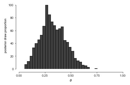
Let’s up \(M\) to \(1\,000\,000\) and double the number of bins to get a better look at the posterior density. ^[A sample size \(M > 100\) is rarely necessary for calculating estimates, event probabilities, or other expectations conditioned on data. For histograms, many draws are required to ensure low relative error in every bin so that the resulting histogram is smooth.]
Histogram of one million draws from the posterior \(p(\theta \mid y)\). A much larger \(M\) is required to get a fine-grained view of the whole posterior distribution than is required for an accurate summary statistic.’}
import numpy as np
import pandas as pd
import matplotlib.pyplot as plt
import seaborn as sns

np.random.seed(1234)
M = 1000000
theta = np.random.beta(y + 1, N - y + 1, M)

binom_post_df2 = pd.DataFrame({'theta': theta})
binomial_post_plot2 = sns.histplot(data=binom_post_df2, x='theta', color='black', fill='#ffffe6', edgecolor='black', bins=60)
binomial_post_plot2.set(xlim=(0, 1), xticks=[0, 0.25, 0.5, 0.75, 1], xlabel=r'$\theta$', ylabel='posterior draw proportion')
sns.set_style('ticks')
sns.despine(offset=10, trim=True)
plt.show()
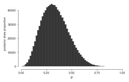
Histograms have their limitations. The distribution is slightly asymmetric, with a longer tail to the right than to the left, but asymmetry can be difficult to detect visually until it is more extreme than here. Asymmetric distributions are said to be skewed, either to the right or left, depending on which tail is longer.^[The formal measurement of the skew of a random variable \(Y\) is just another expectation that may be estimated via simulation, \(\mbox{skew}[Y] = \mathbb{E}\left[\left(\frac{Y - \mathbb{E}[Y]}{\mbox{sd}[Y]}\right)^3\right].\)] It’s also hard to tell the exact location of the posterior mean and median visually.
Posterior summary statistics
We often want to look at summaries of the posterior, the posterior mean, standard deviation, and quantiles being the most commonly used in practice. These are all easily calculated based on the sample draws.
Calculating the posterior mean and standard deviation are as simple as calling built-in mean and standard deviation functions,
print('estimated posterior mean =', np.mean(theta))
print('estimated posterior sd =', np.std(theta))
estimated posterior mean = 0.33331827871568803
estimated posterior sd = 0.1309386704210955
Let’s see what we get.
print(f'estimated posterior mean = {np.mean(theta):.2f}')
print(f'estimated posterior sd = {np.std(theta):.2f}')
estimated posterior mean = 0.33
estimated posterior sd = 0.13
The posterior mean and standard deviation are excellent marginal summary statistics for posterior quantities that have a roughly normal distribution.^[Most posterior distributions we will consider approach normality as more data is observed.] If the posterior distribution has very broad or narrow tails or is highly skewed, standard deviation and mean are less useful.
We can estimate quantiles just as easily, assuming we have built-in functions to compute quantiles.
print('estimated posterior median =', np.quantile(theta, 0.5))
print('estimated posterior central 80 pct interval =', np.quantile(theta, [0.1, 0.9]))
estimated posterior median = 0.3237547839111739
estimated posterior central 80 pct interval = [0.16896885 0.51122413]
Running this produces the following.^[The median is slightly lower than the mean, as they will be in right skewed distributions.]
print(f'estimated posterior median = {np.quantile(theta, 0.5):.2f}')
print(f'estimated posterior central 90 pct interval = ({np.quantile(theta, 0.1):.2f}, {np.quantile(theta, 0.9):.2f})')
estimated posterior median = 0.32
estimated posterior central 90 pct interval = (0.17, 0.51)
The posterior simulations and summaries answer Laplace’s question about the value of \(\theta\), i.e., the proportion of boys born, at least relative to this tiny data set.
We have reported a central 90% interval here. It is a 90% interval in the sense that it is 90% probable to contain the value (relative to the model, as always). We have located that interval centrally in the sense that it runs from the 5% quantile to the 95% quantile.
There is nothing privileged about the width or location of a posterior interval. A value is as likely to be in a posterior interval from the 1% quantile to the 91% quantile, or from the 10% quantile to the 100% quantile. The width is chosen to be convenient to reason about. With a 90% interval, we know roughly nine out of ten values will fall within it, and choosing a central interval gives us an idea of the central part of the distribution.
Estimating event probabilities
To answer the question about whether boys are more prevalent than girls, we need to estimate \(\mbox{Pr}[\theta > 0.5]\), which is straightforward with simulation. As usual, we just count the number of times that the simulated value \(\theta^{(m)} > 0.5\) and divide by the number of simulations \(M\),
print(f'estimated Pr[theta > 0.5] = {np.mean(theta > 0.5):.4f}')
estimated Pr[theta > 0.5] = 0.1137
Running this, we see that with 3 boys in 10 births, the probability boys represent more than 50% of the live births is estimated, relative to the model, to be
print(f'estimated Pr[theta > 0.5] = {np.mean(theta > 0.5):.2f}')
estimated Pr[theta > 0.5] = 0.11
Now let’s overlay the median and central 90% interval.
Histogram of \(1,000,000\) draws from the posterior \(p(\theta \mid y, N) \propto \mbox{binomial}(y \mid N, \theta),\) given \(N = 10, y = 3\). The median (50 percent quantile) is indicated with a dashed line and the boundaries of the central 90 percent interval (5 percent and 95 percent quantiles) are picked out with dotted lines. The proportion of the total area shaded to the right of 0.5 represents the posterior probability that \(\theta > 0.5,\) which is about 11 percent.
import numpy as np
from scipy.stats import beta
import matplotlib.pyplot as plt

# observed data
y = 435
N = 982

# prior
a, b = 1, 1
theta_prior = beta(a, b)

# posterior
M = 10000
theta = beta.rvs(a + y, b + N - y, size=M)
likelihood = beta.pdf(theta, a + y, b + N - y)
posterior = theta_prior.pdf(theta) * likelihood

# summary statistics
post_mean = np.mean(theta)
post_median = np.median(theta)
post_sd = np.std(theta)
post_80ci = np.quantile(theta, [0.1, 0.9])
post_prob = np.mean(theta > 0.5)

# plot posterior distribution
plt.hist(theta, bins=50, density=True, color='lightblue')
plt.axvline(x=post_median, linestyle='--', color='black', linewidth=0.5)
plt.axvline(x=post_80ci[0], linestyle=':', color='black', linewidth=0.5)
plt.axvline(x=post_80ci[1], linestyle=':', color='black', linewidth=0.5)
plt.xlabel(r'$\theta$')
plt.ylabel('Density')
plt.title('Posterior Distribution')
plt.show()

# print summary statistics
print(f'estimated posterior mean = {post_mean:.2f}')
print(f'estimated posterior median = {post_median:.2f}')
print(f'estimated posterior sd = {post_sd:.2f}')
print(f'estimated posterior central 90 pct interval = ({post_80ci[0]:.2f}, {post_80ci[1]:.2f})')
print(f'estimated Pr[theta > 0.5] = {post_prob:.2f}')
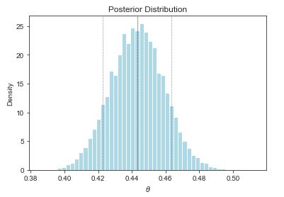
estimated posterior mean = 0.44
estimated posterior median = 0.44
estimated posterior sd = 0.02
estimated posterior central 90 pct interval = (0.42, 0.46)
estimated Pr[theta > 0.5] = 0.00
Laplace’s data
What happens if we use Laplace’s data, rather than our small data set, which had roughly 110 thousand male births and 105 thousand female? Let’s take some draws from the posterior \(p(\theta \mid y, N)\) where \(y = 110\,312\) boys out of \(N = 110\,312 + 105\,287\) total births. We’ll take \(M = 1\,000\,000\) simulations \(\theta^{(1)}, \ldots, \theta^{(M)}\) here because they are cheap and we would like low sampling error.
import numpy as np
import seaborn as sns
import matplotlib.pyplot as plt
from scipy.stats import beta

np.random.seed(1234)

M = 1000000
boys = 110312
girls = 105287
theta = beta.rvs(boys + 1, girls + 1, size=M)

laplace_df = {'theta': theta}
laplace_plot = sns.histplot(data=laplace_df, x='theta', bins=50,
                            color='#ccccb6', edgecolor='black')
laplace_plot.set(xlim=(0.5075, 0.5175), xticks=[0.508, 0.510, 0.512, 0.514, 0.516],
                 xticklabels=['.508', '.510', '.512', '.514', '.516'], xlabel=r'$\theta$',
                 ylabel='posterior draws')
sns.set_style('ticks')
plt.show()
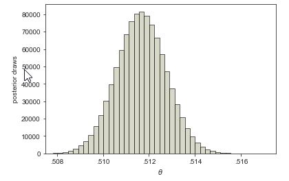
The mean of the posterior sample is approximately 0.511, or a slightly higher than 51% chance of a male birth. The central 90% posterior interval calculated from quantiles of the sample is \((0.510, 0.513)\).
What about the event probability that boy births are more likely than girl births, i.e., \(\mbox{Pr}\[\theta > 0.5\]\)? If we make our usual calculation, taking draws \(\theta^{(1)}, \ldots, \theta^{(M)}\) from the posterior and look at the proportion for which \(\theta^{(m)} > 0.5\), the result is 1. No decimal places, just 1. If we look at the draws, the minimum value of \(\theta^{(m)}\) in \(1\,000,000\) draws was approximately 0.506. The proportion of draws for which \(\theta^{(m)} > 0.5\) is thus 100%, which forms our estimate for \(\mbox{Pr}[\theta > 0.5]\).
As we have seen before, simulation-based estimates provide probabilistic guarantees about absolute tolerances. With \(100\,000\) draws, we are sure that the answer is 1.0000 to within plus or minus 0.0001 or less.^[Tolerances can be calculated using the central limit theorem, which we will define properly when we introduce the normal distribution later.] We know the answer must be strictly less than one. Using some analytic techniques,[The cumulative distribution function of the posterior, which is known to be the beta distribution \(p(\theta \mid y, N) = \mbox{beta}(\theta \mid y + 1, N - y + 1).\)] the true estimate to within 27 decimal places is
[\mbox{Pr}[\theta > 0.5] = 1 - 10^{-27}.]
Thus Laplace was certain that the probability of a boy being born was higher than that of a girl being born.
Inference for and comparison of multiple variables
The first example of Laplace’s is simple in that it has only a single parameter of interest, \(\theta\), the probability of a male birth. Now we will consider a very similar model with two variables, so that we can do some posterior comparisons. We will consider some simple review data for two New York City-based Mexican restaurants. The first contender is Downtown Bakery II, an East Village Mexican restaurant has \(Y_1 = 114\) out of \(N_1 = 235\) 5-star reviews on Yelp, La Delicias Mexicanas, in Spanish Harlem, has \(Y_1 = 24\) out of \(N_2 = 51\) 5-start reviews. Our question is, which is more likely to deliver a 5-star experience? In terms of proportion of 5-star votes, they are close, with Downtown Bakery garnering 49% 5-star reviews and La Delicias only 47%. Knowing how noisy binomial data is, this is too close to call.
We’ll model each restaurant independently for \(n \in 1:2\) as
[Y_n \sim \mbox{binomial}(N, \Theta_n)]
with independent uniform priors for \(n \in 1:2\) as
[\Theta_n \sim \mbox{uniform}(0, 1).]
We can now draw \(\theta^{(1)}, \ldots, \theta^{(M)}\) simulations from the posterior \(p_{\Theta \mid Y, N}(\theta \mid y, N)\) as usual.
The main event is whether \(\theta_1 > \theta_2\)—we want to know if the probability of getting a five-star review is higher at Downtown Bakery than La Delicias. All we need to do is look at the posterior mean of the indicator function \(\mathrm{I}[\theta_1 > \theta_2]\). The calculus gets more complicated—a double integral is now required because there are two variables. The simulation-based estimate, on the other hand, proceeds as before, counting proportion of draws in which the event is simulated to occur.
[\begin{array}{rcl} \mbox{Pr}[\theta_1 > \theta_2 \mid y, N] & = & \int_0^1 \int_0^1 \, \mathrm{I}[\theta_1 > \theta_2] \times p(\theta_1, \theta_2 \mid y, N) \, \mathrm{d} \theta_1 \, \mathrm{d} \theta_2 \[8pt] & \approx & \frac{1}{M} \sum_{m = 1}^M \mathrm{I}[\theta_1^{(m)} > \theta_2^{(m)}]. \end{array}]
In pseudocode, this is just
success = 0
for m in range(M):
    theta_m = posterior.rvs()
    if theta_m > 1 - theta_m:
        success += 1
print(f"Pr[theta[1] > theta[2] | y, M] = {success/M}")
Pr[theta[1] > theta[2] | y, M] = 1.0
Let’s run that with \(M = 10\,000\) simulations and see what we get:
import numpy as np

M = 10000
y = np.array([114, 24])
N = np.array([235, 51])

theta1 = np.random.beta(y[0] + 1, N[0] - y[0] + 1, size=M)
theta2 = np.random.beta(y[1] + 1, N[1] - y[1] + 1, size=M)

prob = np.mean(theta1 > theta2)

print(f"Pr[theta[1] > theta[2] | y, M] = {prob:.2f}")
Pr[theta[1] > theta[2] | y, M] = 0.58
Only about a 52% chance
that Downtown Bakery is the better bet for a 5-star meal.^[As much as
this diner loves Downtown Bakery, the nod for food, ambience, and the
existence of beer goes to La Delicias Mexicanas.]
To get a sense of the posterior, we can construct a histogram of posterior draws of \(\Delta = \Theta_1 - \Theta_2\).
Histogram of posterior differences between probability of Downtown Bakery getting a 5-star review (\(\theta_1\)) and that of La Delicias Mexicanas getting one (\(\theta_2\)). The draws for which \(\delta > 0\) (equivalently, \(\theta_1 > \theta_2\)) are shaded darker. The area of the darker region divided by the total area is the estimate of the probability that Downtown Bakery is more likely to get a 5-star review than La Delicias Mexicanas.
There is substantial uncertainty, and only 52% of the draws lie to the right of zero. That is,
[\mbox{Pr}[\theta_1 > \theta_2] \ = \ \mbox{Pr}[\delta > 0] \ \approx \ 0.52.]
Key Points
Rejection Sampling
Overview
Teaching: min
Exercises: minQuestions
Objectives
Rejection Sampling
Inverse cumulative distribution generation
We have so far assumed we have a uniform random number generator that can sample from a \(\mbox{uniform}(0, 1)\) distribution. That immediately lets us simulate from a \(\mbox{uniform}(a, b).\)^[If \(U \sim \mbox{uniform}(0, 1)\) then \(a + U \times (b - a) \sim \mbox{uniform}(a, b).\)] But what if we want to simulate realizations of a random variable \(Y\) whose density \(p_Y\) is not uniform?
If we happen to have a random variable \(Y\) for which we can compute the inverse \(F^{-1}_Y(p)\) of the cumulative distribution function for \(p \in (0, 1),\)^[If \(F^{-1}_Y(p) = y\) then \(F^{-1}(y) = \mbox{Pr}[Y \leq y] = p.\)] then we can simulate random realizations of \(Y\) as follows. First, simulate a uniform draw \(U\),
[u^{(m)} \sim \mbox{uniform}(0, 1),]
then apply the inverse cumulative distribution function to turn it into a simulation of \(Y\),
[y^{(m)} = F^{-1}(u^{(m)}).]
It turns out we’ve already seen an example of this strategy—it is how we simulated from a logistic distribution right off the bat. The log odds transform is the inverse cumulative distribution function for the logistic distribution. That is, if
[Y \sim \mbox{logistic}(0, 1),]
then
[F_Y(y) = \mbox{logit}^{-1}(y) = p]
and hence
[F^{-1}_Y(p) = \mbox{logit}(p) = y.]
This lets us simulate \(Y\) by first simulating \(U \sim \mbox{uniform}(0, 1)\), then setting \(Y = \mbox{logit}(U)\). Both the log odds function and its inverse are easy to compute. Often, the inverse cumulative distribution function is an expensive computation.^[In general, the inverse cumulative distribution function \(F^{-1}_Y(p)\) can be computed by solving \(F_Y(u) = \int_{\infty}^u p_Y(y) \, \mathrm{d} y = p\) for \(u\), which can typically be accomplished numerically if not analytically.]
Beta distribution
As a first non-trivial example, let’s consider the beta distribution, which arises naturally as a posterior in binary models. Recall that when we have a binomial likelihood \(\mbox{binomial}(y \mid N, \theta)\) and a uniform prior \(\theta \sim \mbox{uniform}(0, 1)\), then the posterior density is
[p(\theta \mid y)
\ \propto
\theta^y \times (1 - \theta)^{N - y}.]
This turns out to be a beta distribution with parameters \(\alpha = y + 1\) and \(\beta = N - y + 1\). If a random variable \(\Theta \in (0, 1)\) has a beta distribution, then its density \(p_{\Theta}\) is
[\mbox{beta}(\theta \mid \alpha, \beta)
\ \propto
\theta^{\alpha - 1} \times (1 - \theta)^{\beta - 1}]
for some \(\alpha, \beta > 0\).^[We prefer to present densities up to normalizing constants, because the normalizing constants are distracting—what matters is how the density changes with the variate. Here, the fully normalized distribution is \(\mbox{beta}(\theta \mid \alpha, \beta) \ = \ \frac{1}{\mbox{B}(\alpha, \beta)} \, \theta^{\alpha - 1} \times (1 - \theta)^{\beta - 1},\) where Euler’s beta function, which gives its namesake distribution its name, is defined as the integral of the unnormalized beta density \(\mathrm{B}(\alpha, \beta) \ = \ \displaystyle \int_0^1 \theta^{\alpha - 1} (1 - \theta)^{\beta - 1} \, \mbox{d} \theta.\) Hence, it’s clear the beta density integrates to 1 for any \(\alpha, \beta\).]
If \(Y \sim \mbox{beta}(\alpha, \beta)\), then its expected value is
[\mathbb{E}[Y] = \frac{\alpha}{\alpha + \beta}.]
It is convenient to work with the beta distribution parameters in terms of the mean \(\alpha / (\alpha + \beta)\) and the total count \(\alpha + \beta\).^[Distributions have means, random variables have expectations. The mean of a distribution is the expectation of a random variable with that distribution, so the terms are often conflated.] The higher the total count, lower the variance. For example, here is a plot of a few beta distributions organized by total count and mean.
import pandas as pd
import numpy as np
import matplotlib.pyplot as plt
from scipy.stats import beta
import seaborn as sns

# Create empty dataframes to store results
beta_density_df = pd.DataFrame(columns=['theta', 'p_theta', 'count', 'mean'])
mean_df = pd.DataFrame(columns=['expectation', 'count', 'mean'])

# Define thetas and iterate over combinations of kappa and mu
thetas = np.arange(0, 1.01, 0.01)
for kappa in [0.5, 2, 8, 32]:
    for mu in [0.5, 0.675, 0.85]:
        p_theta = beta.pdf(thetas, kappa * mu, kappa * (1 - mu))
        df_temp = pd.DataFrame({'theta': thetas,
                                'p_theta': p_theta,
                                'count': ['count ' + str(kappa)] * len(thetas),
                                'mean': ['mean ' + str(mu)] * len(thetas),
                                'mu': [mu] * len(thetas)})
        beta_density_df = pd.concat([beta_density_df, df_temp])

# Create the beta density plot
beta_density_plot = sns.relplot(x='theta', y='p_theta', kind='line', col='count', row='mean',
                                data=beta_density_df, facet_kws={'sharex': True, 'sharey': True},
                                height=2.5, aspect=1.5)

# Add vertical lines at mu
for ax in beta_density_plot.axes.flat:
    ax.axvline(mu, ls=':', lw=0.5)

# Format plot
beta_density_plot.set(xlim=(0, 1), ylim=(0, 7))
beta_density_plot.set(xticks=[0, 0.5, 1], xticklabels=['0', '0.5', '1'])
beta_density_plot.set(yticks=[0, 3, 6])
beta_density_plot.set_axis_labels(r'$\theta$', r'$\beta(\theta|\alpha,\beta)$')
beta_density_plot.fig.subplots_adjust(wspace=0.3, hspace=0.3)
sns.set_theme(style='ticks')

plt.show()
Plots of the densities
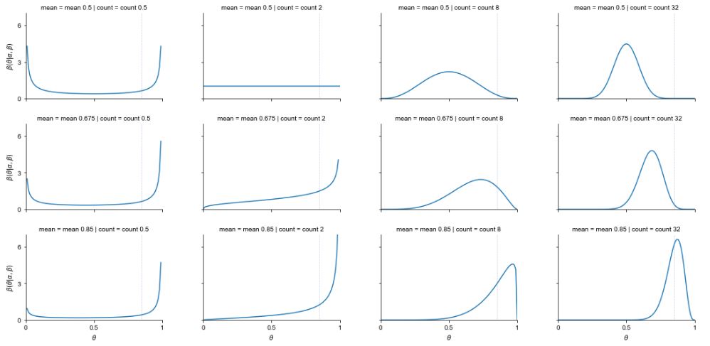
For example, a total count of \(\alpha + \beta = 8\) and mean of \(\alpha / (\alpha + \beta) = 0.85\) corresponds to beta distribution parameters \(\alpha = 8 \times 0.85 = 6.8\) and \(\beta = 8 \times (1 - 0.85) = 1.2.\)
The plot shows that when the mean is 0.5 and the count is 2 (i.e., \(\alpha = \beta = 1\)), the result is a uniform distribution. The algebra agrees,
[\begin{array}{rcl} \mbox{beta}(\theta \mid 1, 1) & \propto & \theta^{1 - 1} \times (1 - \theta)^{1 - 1} \[4pt] & = & 1 \[4pt] & = & \mbox{uniform}(\theta \mid 0, 1). \end{array}]
The area under each of these curves, as drawn, is exactly one. The beta distributions with small total count (\(\alpha + \beta\)) concentrate most of their probability mass near the boundaries. As the count grows, the probability mass concentrates away from the boundaries and around the mean.^[Nevertheless, in higher dimensions, the curse of dimensionality rears its ugly head, and concentrates the total mass in the corners, even if each dimension is independently distributed and drawn from a distribution concentrated away from the edges in one dimension. The reason is the same—each dimension’s value squared just pulls the expected distance of a draw further from the multidimensional mean.]
Each of these distributions has a well-defined mean, as shown in row labels in the plot. But they do not all have well defined modes (maxima). For example, consider the beta distribution whose density is shown in the upper left example in the plot. It shows a U-shaped density for a \(\mbox{beta}(0.25, 0.25)\) distribution, which corresponds to mean \(0.5 = 0.25 / (0.25 + 0.25)\) and total count \(0.5 = 0.25 + 0.25\). As \(\theta\) approaches either boundary, 0 or 1, the density grows without bound. There is simply no maximum value for the density.^[Despite the lack of a maximum, the area under the density is one. The region of very high density near the boundary becomes vanishingly narrow in order to keep the total area at one.]
Uniform, bounded rejection sampling
How do we sample from a beta distribution? Rejection sampling is a very simple algorithm to sample from general distributions for which we know how to compute the density. It is a good starter algorithm because it is easy to understand, but points the way toward more complex sampling algorithms we will consider later.
Let’s start with the simplest possible kind of rejection sampling where we have a bounded distribution like a beta distribution. The values drawn from a beta distribution are bounded between 0 and 1 by construction. Furthermore, if \(\alpha, \beta > 1\), as we will assume for the time being, then there is a maximum value for \(\mbox{beta}(\theta \mid \alpha, \beta)\).^[The maximum density occurs at the mode of the distribution, which for \(\textrm{beta}(\theta \mid \alpha, \beta)\) is given by \(\theta^* = \frac{\alpha - 1}{\alpha + \beta - 2}.\)]
For concreteness, let’s start specifically with a \(\mbox{beta}(6.8, 1.2)\) distribution, corresponding to the mean 0.85 and count of 8 case from the previous section. We observe that all values fall below 5, so we will create a box with height 5 and width of 1.^[For an unknown distribution, we could use an optimization algorithm to find the largest value.] Next, we draw uniformly from the box, drawing a horizontal position \(\theta^{(m)} \sim \mbox{uniform}(0, 1)\) and vertical position \(u^{(m)} \sim \mbox{uniform}(0, 5)\). The points whose value for \(u\) falls below the density at the value for \(\theta\) are retained.
import numpy as np
import pandas as pd
import matplotlib.pyplot as plt
from scipy.stats import beta
import seaborn as sns

M = 500
alpha = 6.8
beta_value = 1.2
mean = alpha / (alpha + beta_value)
mode = (alpha - 1) / (alpha + beta_value - 2)
y = np.arange(0, 1.01, 0.01)
u = np.random.uniform(0, 5, size=M)
theta = np.random.uniform(0, 1, size=M)
accept = (u < beta.pdf(theta, alpha, beta_value))

reject_beta_df = pd.DataFrame({'y': y, 'p_y': beta.pdf(y, alpha, beta_value)})
accept_beta_df = pd.DataFrame({'theta': theta, 'u': u, 'accept': accept})

reject_beta_plot = sns.lineplot(x='y', y='p_y', data=reject_beta_df)
reject_beta_plot.set(xlabel=r'$\theta$', ylabel=r'$p(\theta)$')
reject_beta_plot.axhline(y=0, linestyle='--', color='k')
reject_beta_plot.axhline(y=5, linestyle='--', color='k')
reject_beta_plot.axvline(x=0, linestyle='--', color='k')
reject_beta_plot.axvline(x=1, linestyle='--', color='k')

accept_plot = sns.scatterplot(x='theta', y='u', hue='accept', data=accept_beta_df, s=20, alpha=0.8)
accept_plot.set(xlabel=r'$\theta$', ylabel='u')
accept_plot.axhline(y=0, linestyle='--', color='k')
accept_plot.axhline(y=5, linestyle='--', color='k')
accept_plot.axvline(x=0, linestyle='--', color='k')
accept_plot.axvline(x=1, linestyle='--', color='k')
A simple instance of rejection sampling from a bounded \(\mbox{beta}(6.8, 1.2)\) distribution, whose density is shown as a solid line. Points \((\theta, u)\) are drawn uniformly from the rectangle, then accepted as a draw of \(\theta\) if \(u\) falls below the density at \(\theta\). The accepted draws are rendered as plus signs and the rejected ones as circles. The acceptance rate here is roughly 20 percent.
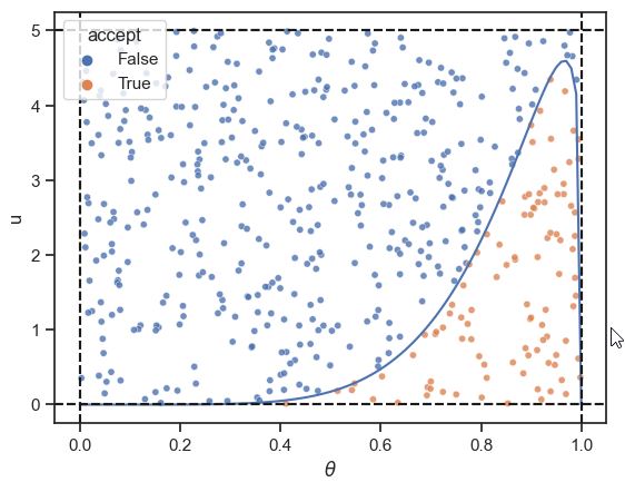 More specifically, we keep the values \(\theta^{(m)}\) where
[u^{(m)} < \mbox{beta}(\theta^{(m)} \mid 6.8, 1.2).]
The set of accepted draws that are retained are distributed uniformly in the area under the density plot. The probability of a draw from rejection sampling for variable \(U\) falling between points \(a\) and \(b\) is proportional to the area under the density curve between \(a\) and \(b\), which is the correct probability by the definition of the probability density function \(p_U\), which ensures
[\mbox{Pr}[a \leq U \leq b] = \int_a^b p_U(u) \, \mathrm{d}u.]
If the intervals are right, the density is right.
Rejection sampling algorithm
To generate a single draw from \(\mbox{beta}(6.8, 1.2)\), we continually sample points \((u, \theta)\) uniformly until we find one where \(u\) falls below the density value for \(\theta\), then return the \(\theta\) value. Because the variable \(u\) is only of use for sampling, it is called an auxiliary variable. Many sampling methods use auxiliary variables. The rejection sampling algorithm written out for our particular case is as follows.
import numpy as np
from scipy.stats import beta

while True:
    u = np.random.uniform(0, 5)
    theta = np.random.uniform(0, 1)
    if u < beta.pdf(theta, 6.8, 1.2):
        break
Let’s run this algorithm for \(M = 100\,000\) iterations and see what the histogram looks like.
import numpy as np
import pandas as pd
import matplotlib.pyplot as plt
from scipy.stats import beta
import seaborn as sns
np.random.seed(1234)

M = 100000
accept = 0
total = 0
m = 1
theta = np.empty(M)
while m <= M:
    u = np.random.uniform(0, 5)
    theta_star = np.random.uniform(0, 1)
    total += 1
    if u < beta.pdf(theta_star, 6.8, 1.2):
        accept += 1
        theta[m-1] = theta_star
        m += 1
beta_draws_df = pd.DataFrame({'theta': theta})
beta_draws_plot = sns.histplot(data=beta_draws_df, x='theta', stat='density', bins=80, color='black', fill='#ffffe8', kde=True, alpha=0.8)
beta_draws_plot.set(xlabel=r'$\theta$', ylabel=r'$p(\theta)$')
beta_draws_plot.axvline(x=0, linestyle='--', color='k')
beta_draws_plot.axvline(x=1, linestyle='--', color='k')
beta_draws_plot.plot(np.linspace(0, 1, 100), beta.pdf(np.linspace(0, 1, 100), 6.8, 1.2), color='black', linewidth=0.35)
print(f"acceptance percentage = {accept/total:.2%}")
Histogram of \(M = 100,000\) Draws from \(\mbox{beta}(6.8, 1.2)\) made via rejection sampling. The true density is plotted over the histogram as a line. The acceptance rate for draws was roughly 20 percent.
acceptance percentage = 20.06%
.jpg)
This looks like it’s making the appropriately distributed draws from the beta distribution.^[After we introduce the normal distribution, we will develop a \(\chi^2\) test statistic for whether a given set of draws come from a specified distribution. For now, we perform the inaccurate test known informally as “\(\chi\) by eye.”]
Acceptance, concentration, and the curse of dimensionality
As noted in the caption of the plot, the acceptance rate is only 20% for the uniform proposals. This acceptance rate can become arbitrarily bad with uniform proposals as the true distribution from which we want to sample concentrates around a single value. As such, rejection sampling’s value is as a pedagogical example for introducing generic sampling and also as a component in more robust sampling algorithms.
The algorithm could also be extended to higher dimensions, but the problem of rejection becomes worse and worse due to the curse of dimensionality. If the posterior is concentrated into a reasonably small area (even as mildly in our \(\mbox{beta}(6.8, 1.2)\) example) in each dimension, the chance of a random multidimensional sample being accepted in every dimension is only \(0.2^N\), which becomes vanishingly small for practical purposes even in 10 dimensions.^[In ten dimensions, overall acceptance of a uniform draw would be \(0.2^{10}\), or a little less than one in ten million. While this may be possible with patience, another ten dimensions becomes completely unworkable, even with massive parallelism.]
General rejection sampling
The more general form of rejection sampling takes a proposal from an arbitrary scaled density. In the example of the previous section, we used a \(\mbox{uniform}(0, 1)\) distribution scaled by a factor of five. The acceptance procedure in the general case remains exactly the same.
In the general case, suppose we want to draw from a density \(p(y)\). We’ll need a density \(q(y)\) from which we know how to simulate draws, and we’ll need a constant \(c\) such that
[c \times q(y) > p(y)]
for all \(y\).^[This means the support of the proposal distribution must be at least as large as that of the target distribution.]
The general rejection sampling algorithm for target density \(p(y)\), proposal density \(q(y)\) with constant \(c\) such that \(c \times q(y) > p(y)\) for all \(y\), is as follows:
while True:
    y = q_rng(y)
    u = np.random.uniform(0, c*q(y))
    if u < p(y):
        return y
Our simplified algorithm in the previous section was just a special case where \(q(y)\) is uniform over a bounded interval. The argument for correctness in the more general case is identical—draws are made proportional to the area under the density, which provides the correct distribution.
Key Points
Conjugate Posteriors
Overview
Teaching: min
Exercises: minQuestions
Objectives
Posterior Predictive Inference
One of the primary reasons we fit models is to make predictions about the future. More specifically, we want to observe some data \(y\) and use it to predict future data \(\tilde{y}\). Even more specifically, we’d like to understand the probability distribution of the future data \(\tilde{y}\) given the observed data \(y\).
We are going to assume that we are still working relative to a model whose sampling distribution has a density \(p(y \mid \theta)\).^[From now on, we’ll be dropping random variable subscripts on probability functions. The convention in applied statistics is to choose names for bound variables that allow the random variables to be determined by context. For example, we will write \(p(\theta \mid y)\) for a posterior, taking it to mean \(p_{\Theta \mid Y}(\theta \mid y)\).] Thus if we knew the value of \(\theta\),^[We are also overloading lowercase variables like \(\theta\) to mean their random variable counterpart \(\Theta\) when necessary, as it is here, where we should properly be saying that the random variable \(\Theta\) takes on some known value \(\theta\).] the distribution of \(\tilde{y}\) would be given by \(p(\tilde{y} \mid \theta)\). Here, we are assuming that the sampling distribution will be the same density for the original data \(p(y \mid \theta)\) and the predictive data \(p(\tilde{y} \mid \theta)\).
Unfortunately, we don’t know the true value of \(\theta\). All we have to go on are the inferences we can make about \(\theta\) given our model and observed data \(y\). As we saw in the last chapter, this knowledge is encapsulated in a posterior distribution with density \(p(\theta \mid y)\). So rather than making predictions \(p(\tilde{y} \mid \theta)\) based on a single estimated value of \(\theta\), we are going to create a weighted average of predictions for every possible \(\theta\) with weights determined by the posterior \(p(\theta \mid y)\). Because \(\theta\) is continuous, the averaging must proceed by integration. The result is the posterior predictive distribution, the density for which is defined by
[p(\tilde{y} \mid y)
\ =
\displaystyle
\int_{\Theta}
p(\tilde{y} \mid \theta)
\times
p(\theta \mid y)
\,
\mathrm{d}\theta.]
The variable \(\Theta\) is now doing extra duty as the set of possible values for \(\theta\), that is the range of variables over which \(\theta\) is averaged.
When estimating the probability of new data, there are two forms of uncertainty that need to be taken into account. The first is estimation uncertainty arising from not knowing the exact value of \(\theta\). This comes into play by averaging over the posterior \(p(\theta \mid y)\). The second form of uncertainty is introduced by the sampling distribution \(p(\tilde{y} \mid \theta)\). Even if we knew the precise value of \(\theta\), we would still not know the value of \(\tilde{y}\) because it is not a deterministic function of \(\theta\). Let’s write our formula again highlighting the two sources of uncertainty.
[p(\tilde{y} \mid y)
\ =
\int_{\Theta}
\underbrace{p(\tilde{y} \mid \theta)}{\mbox{sampling uncertainty}}
\times
\underbrace{p(\theta \mid y)}{\mbox{estimation uncertainty}}
\,
\mathrm{d}\theta.]
Calculation via simulation
The probability mass function for the posterior predictive is defined by an integral that averages over the posterior, thus it can be estimated using simulations \(\theta^{(1)}, \theta^{(M)}\) of the posterior \(p(\theta \mid y)\) as
[p(\tilde{y} \mid y)
\ \approx
\frac{1}{M} \sum_{m=1}^M p(\tilde{y} \mid \theta^{(m)}).]
That is, we just take the average prediction over our sample of simulations.
Continuing our example from the previous chapter, we will put everything together and show how to compute posterior predictive densities. To review, we have \(y\) boys born out of \(N\) births, under the sampling distribution \(y \sim \mbox{binomial}(N, \theta)\) and prior \(\theta \sim \mbox{uniform}(0, 1)\). We have shown in the previous chapter how to take simulated draws \(\theta^{(1)}, \ldots, \theta^{(M)}\) from the posterior distribution with density \(p(\theta \mid y, N)\).
Now suppose we have new data \(\tilde{y}\) from a trial of size \(\tilde{N}\). We can estimate \(p(\tilde{y} \mid y, \tilde{N})\) by instantiating the general formula above,
[p(\tilde{y} \mid y, \tilde{N})
\ \approx
\frac{1}{M} \sum_{m = 1}^M
\mbox{binomial}(\tilde{y} \mid \tilde{N}, \theta^{(m)}).]
If we treat \(\mbox{binomial}\) as evaluating elementwise,^[A function \(f : \mathbb{R} \rightarrow \mathbb{R}\) can be extended elementwise to a function on sequences \(f : \mathbb{R}^N \rightarrow \mathbb{R}^N\) by defining \(f(x)[n] = f(x[n]).\) For example, elementwise exponentiation satisfies \(\exp((u, v, w)) = (\exp(a), \exp(v), \exp(w)).\)] so that a collection of \(\theta\) as input produces a collection as output, then we can write this using the elementwise definition of the binomial and a function to calculation the mean of a collection as
[\begin{array}{rcl} p!\left(\tilde{y} \mid y\right) & \approx & \mbox{mean}!\left(\mbox{binomial}!\left(\tilde{y} \mid \tilde{N}, \theta\right)\right). \[6pt] & \approx & \mbox{mean}!\left(\mbox{binomial}!\left(\tilde{y} \mid \tilde{N}, \left(\theta^{(1)}, \ldots \theta^{(M)}\right)\right)\right). \[6pt] & = & \mbox{mean}!\left( ( \mbox{binomial}!\left(\tilde{y} \mid \tilde{N}, \theta^{(1)}\right), \ldots, \mbox{binomial}!\left(\tilde{y} \mid \tilde{N}, \theta^{(M)}\right) \right) \[6pt] & = & \frac{1}{M} \sum_{m=1}^M \mbox{binomial}!\left(\tilde{y} \mid \tilde{N}, \theta^{(m)}\right). \end{array}]
The second two lines illustrate how an elementwise definition is expanded, and the third shows how the compound function for the mean is applied.^[The definition of the mean function is \(\mbox{mean}\!\left( (u_1, \ldots, u_N) \right) \ = \ \frac{1}{N} \sum_{n=1}^N u_n.\)]
The pseudocode translates the mathematical definition directly.
for (m in 1:M)
  draw theta(m) from posterior p(theta | y, N)
  p[m] = binomial(y_pred | N_pred, theta(m))
print 'esimated p(y_pred | y) = ' mean(p)
With an elementwise version of the binomial probability mass function, this simplifies to the following.^[Simple can mean several things—we’re measuring code simplicity, not necessarily how simple it is to undersetand. Code simplicity involves several things, among them shallower nesting of statments and fewer indexed expressions, as in this example. As another example, the calculation of the mean could be done manually, but it is simpler to use a library function. Even if there’s no library function, it simplifies code to break complex operations down into well-named functions. Building up a personal library of such functions is the first step toward becoming a developer.]
for (m in 1:M)
  draw theta(m) from posterior p(theta | y, N)
p = binomial(y_pred | N_pred, theta)
print 'estimated p(y_pred | y) = ' mean(p)
Let’s continue with the small data example, where \(y = 3\) and \(N = 10\). We’ll take \(\tilde{N} = 20\) in order to make a prediction over the next twenty observations and calculate the probability for each possible \(\tilde{y} \in 0:\tilde{N}\). Then we’ll plot them in a bar chart to inspect the distribution.
```{r fig.cap = ‘Probability mass function for the posterior predictive distribution of the number of boys, \(\\theta^{*} = \\frac{y}{N} = 0.3\), into the sampling distribution, to yield \(\\mbox{binomial}(\\tilde{y} \\mid \\tilde{N}, \\theta^{*})\). Compared to the full posterior taking into account estimation uncertainty in \(\\theta\), this plug-in estimate makes it seem very unlikely there will be more boys than girls born in the next 20 births.’}
set.seed(1234) log_sum_exp <- function(u) max(u) + log(sum(exp(u - max(u)))) M <- 1000 y <- 3 N <- 10 N_pred <- 20 lp <- rep(NA, M) log_pred <- rep(NA, N_pred + 1) theta <- rbeta(M, y + 1, N - y + 1) for (y_pred in 0:N_pred) { for (m in 1:M) { lp[m] <- dbinom(y_pred, N_pred, theta[m], log = TRUE) } log_pred[y_pred + 1] <- log_sum_exp(lp) - log(M) }
pp3_10_df <- data.frame(y_pred = 0:20, log_p = exp(log_pred)) pp1_plot <- ggplot(pp3_10_df, aes(y_pred, log_p)) + geom_col(color=’black’, fill = ‘#ffffe8’, size = 0.25) + xlab(expression(widetilde(y))) + ylab(expression(paste(“p(“, widetilde(y), “ | “, y, “)”))) + ggtheme_tufte() pp1_plot
Because we have only observed $$N$$ outcomes, the posterior is not very
concentrated---it is consistent with a wide range of possible
outcomes. Contrast this situation to using the binomial directly to do
prediction by setting $$\theta = 0.3$$, the observed proportion of
boys.^[Inference with a single point estimate of one or more
parameters is common in live, real-time applications, where the cost
of averaging over the posterior may be prohibitive.]

```{r fig.cap = 'Probability mass function for predictions made by plugging the proportion of boy births observed in the data  $$\\tilde{y}$$ in a subsequent group of $$\\tilde{N} = 20$$ births based on observing 3 boys in 10 births with no prior information.  Although it is peaked near the 30 percent level observed in the data, it would not be that surprising to see more boys than girls in the next 20 births.'}

binom_df <- data.frame(y_pred = 0:20, log_p = dbinom(0:20, 20, 0.3))
binom_plot <-
  ggplot(binom_df, aes(y_pred, log_p)) +
  geom_col(color='black', fill = '#ffffe8', size = 0.25) +
  xlab(expression(widetilde(y))) +
  ylab(expression(paste("binom(", widetilde(y), " |", widetilde(N), ", 0.3)"))) +
  ggtheme_tufte()
binom_plot
The probability mass in the predictions is much more concentrated around the observed proportion of boys. Ignoring the estimation uncertainty in \(\theta\) captured by the full posterior leads to inferences that are overly concentrated compared to the full probabilistic conditioning on observed data. As we will see in subsequent chapters, such predictions are not well calibrated for future data assuming the model is correct—they place too much certainty in the observed proportion of boys in a small sample.
The full posterior automatically adjusts for the size of the sample. Consider the following plot, in which the same proportion of boys is provided (30%), but the sample size continues to grow (quadrupling each time).
```{r out.width = “100%”, fig.width = 9, fig.asp=0.4, fig.cap = ‘Illustration of convergence of posterior to binomial prediction based on proportion of boys as number of observations \(y\) and \(N\) grows, with proportion \(\\frac{y}{N}\) fixed. The central limit theorem tells us that each quadrupling of the data cuts the uncertainty in parameter estimation in half until all that is left is the sampling uncertainty in the binomial, as represented in the final plot, where \(\\theta = 0.3\) is fixed.’}
M <- 1000
y <- 12 N <- 40 N_pred <- 20 lp <- rep(NA, M) log_pred <- rep(NA, N_pred + 1) theta <- rbeta(M, y + 1, N - y + 1) for (y_pred in 0:N_pred) { for (m in 1:M) { lp[m] <- dbinom(y_pred, N_pred, theta[m], log = TRUE) } log_pred[y_pred + 1] <- log_sum_exp(lp) - log(M) } pp12_40_df <- data.frame(y_pred = 0:20, log_p = exp(log_pred))
y <- 48 N <- 160 N_pred <- 20 lp <- rep(NA, M) log_pred <- rep(NA, N_pred + 1) theta <- rbeta(M, y + 1, N - y + 1) for (y_pred in 0:N_pred) { for (m in 1:M) { lp[m] <- dbinom(y_pred, N_pred, theta[m], log = TRUE) } log_pred[y_pred + 1] <- log_sum_exp(lp) - log(M) } pp48_160_df <- data.frame(y_pred = 0:20, log_p = exp(log_pred))
pp_full_df <- data.frame(y_pred = c(), log_p = c(), model = c()) pp_full_df <- rbind(pp_full_df, data.frame(y_pred = pp3_10_df\(y_pred, log_p = pp3_10_df\)log_p, model = rep(paste(‘y = 3, N = 10’), 21))) pp_full_df <- rbind(pp_full_df, data.frame(y_pred = pp12_40_df\(y_pred, log_p = pp12_40_df\)log_p, model = rep(paste(‘y = 12, N = 40’), 21))) pp_full_df <- rbind(pp_full_df, data.frame(y_pred = pp48_160_df\(y_pred, log_p = pp48_160_df\)log_p, model = rep(paste(‘y = 48, N = 160’), 21))) pp_full_df <- rbind(pp_full_df, data.frame(y_pred = binom_df\(y_pred, log_p = binom_df\)log_p, model = rep(‘fix theta = 0.3’, 21)))
pp_full_plot <- ggplot(pp_full_df, aes(y_pred, log_p)) + facet_grid(cols = vars(model)) +
facet_wrap( ~ model) +
geom_col(color=’black’, fill = ‘#ffffe8’, size = 0.1) + xlab(expression(widetilde(y))) + ylab(‘probability’) + ggtheme_tufte() + theme(panel.spacing.x = unit(1, “lines”)) pp_full_plot
As the data size grows, the posterior predictive distribution
approaches the predictions derived from just plugging the proportion
of boys observed (30%) in the sampling distribution. After 160
observations, the posterior predictive distribution is only a percent
or two away from the predictions that do not take into account
estimation uncertainty. Whether that matters or not will depend on the
application.^[If leveraged bets or lives are at stake, a 1%
discrepancy in predictions can have enormous consequences.]

## Numerically stable expectations on the log scale

We often run into the problem of underflow when computing densities or
probabilities.^[Underflow is the result of operations which produce
real numbers $$\epsilon$$ smaller than the smallest number that can
be represented.]  To get around that problem we compute on the log
scale, using $$\log p(y \mid \theta)$$ rather than doing calculations on
the original scale $$p(y \mid \theta)$$.

But we have to be careful with averaging non-linear operations.  The
averaging that we do with simulation-based estimates does not
distribute.  For most $$u$$ and $$v$$,^[An exception is $$u = v = 2.$$]

$$
\log u + \log v \neq \log (u + v).
$$

As a result, the log of an average is not equal to the average of a
log,

$$
\frac{1}{M} \sum_{m=1}^M \log u_m
\neq
\log \left( \frac{1}{M} \sum_{m = 1}^M u_m \right).
$$

All is not lost, however.  We will rewrite our desired result as

$$
\begin{array}{rcl}
\log \frac{1}{M} \sum_{m = 1}^M p(\tilde{y} \mid \theta^{(m)})
& = &
\log \frac{1}{M} + \log \sum_{m = 1}^M p(\tilde{y} \mid \theta^{(m)})
\\[4pt]
& = &
- \log M
+ \log \sum_{m=1}^M \exp
     \left( \log p(\tilde{y} \mid \theta^{(m)}) \right)
\\[4pt]
& = &
\mbox{log\_sum\_exp}(\log p(\tilde{y} \mid \theta)) - \log M.
\end{array}
$$

Extending our example, we can work on the log scale to stabilize
calculations with larger $$N$$ by calculating

$$
\begin{array}{rcl}
\log p(\tilde{y} \mid y)
& \approx &
\log \sum_{m=1}^M
\exp\left(
\log \mbox{binomial}(\tilde{y} \mid \tilde{N}, \theta^{(m)})
\right).
\\[8pt]
& = &
\mbox{log\_sum\_exp}(\log \mbox{binomial}(\tilde{y} \mid \tilde{N}, \theta)).
\end{array}
$$

As with the algorithm on the original scale, the pseudocode is
straightforward given a means to draw $$\theta^{(m)}$$ from the
posterior $$p(\theta \mid y, N)$$.^[Typically, software will have the
binomial implemented on the log scale directly, so it won't be
necessary to take the log of the standard scale version.]
for (m in 1:M) draw theta(m) from posterior p(theta | y, N) lp[m] = log(binomial(y_pred | N_pred, theta(m)) print ‘log p(y_pred | y) = ‘ log_sum_exp(lp) ```
Thus we can calculate posterior predictive densities on the log scale using log scale density calculations throughout to prevent overflow and underflow in intermediate calculations or in the final result.
Posterior predictive densities as expectations
Working with expectations and conditional expectations is natural for posterior inference, but initially requires some mental gymnastics to interpret all the implicit bindings. Using expectation notation, the posterior predictive distribution can be defined as
[p(\tilde{y} \mid y)
\ =
\displaystyle
\mathbb{E}!\left[ p(\tilde{y} \mid \theta) \mid y \right].]
We are now overloading lower case variables to do double duty as their upper-case counterparts. Rendered with full random variable indexing, the expectation and its definition are
[\begin{array}{rcl} p_{\tilde{Y} \mid Y}(\tilde{y} \mid y) & = & \displaystyle \mathbb{E}!\left[ p_{\tilde{Y}\mid\Theta}(\tilde{y} \mid \Theta) \mid Y = y \right] \[8pt] & = & \displaystyle \int_T p_{\tilde{Y}\mid\Theta}(\tilde{y} \mid \theta) \times p_{\Theta \mid Y}(\theta \mid y) \, \mathrm{d} \theta, \end{array}]
where \(T\) is domain of integration for \(\theta\), i.e., possible values for \(\Theta\). The twist is that the function whose expectation is being taken is now a density \(p(\tilde{y} \mid \theta)\) in which \(\theta\) shows up as a conditioning variable for the data \(\tilde{y}\) being predicted.
The trick to understanding expectations is in understanding which variables are bound—all other random variables are averaged out to define the expectation. The value of both the observed data \(y\) and the data \(\tilde{y}\) for which we are computing predictions are fixed by the function definition and are not free variables in the expectation. The random variable \(\theta\) is not bound anywhere, and hence it is averaged in the calculation.
Key Points
Floating Point Arithmetic
Overview
Teaching: min
Exercises: minQuestions
Objectives
Floating Point Arithmetic
Contemporary^[Contemporary being 2019 as of this writing.] computers use floating-point representations of real numbers and thus perform arithmetic on floating-point representations.
What is a floating point number?
A bit is the smallest discrete representational unit in a computer—it takes on a value of 0 or 1.^[A byte consists of a sequence of 8 bits. The natural computing unit is a word, the size of which is hardware dependent, but most computers nowadays (it’s still 2019) use 64-bit, or 8-byte words.] Floating point numbers are most commonly represented using 32 or 64 bits, which are known as single precision and double precision respectively.^[Modern machine learning floating point representations go as low as 8 bits and high-precision applied mathematical calculations may use 1024 bits or more.]
Finite, not-a-number, and infinite values
A floating point number consists of a fixed number of bits for a significand \(a\) and a fixed number of bits for the exponent \(b\) to represent the real number \(a \times 2^b\). The significand determines the precision of results and the exponent the range of possible results.^[This exponent causes the decimal place to float, giving the representation its name.] The significand may be negative in order to represent negative values. The exponent may be negative in order to represent fractions. Both the significand and exponent are represented using a single bit for a sign and the remaining bits for the value in binary representation. Standard double-precision (i.e., 64 bit) representations allocate 53 bits for the significand and 11 bits for the exponent.^[Zuras, D., Cowlishaw, M., Aiken, A., Applegate, M., Bailey, D., Bass, S., Bhandarkar, D., Bhat, M., Bindel, D., Boldo, S. and Canon, S., 2008. *IEEE Standard 754-2008 (floating-point arithmetic).]
The standard also sets aside three special values, not a number for ill-defined results, e.g., dividing zero by zero, positive infinity for infinite results, e.g., dividing one by zero, and negative infinity for negative infinity, e.g., dividing negative one by zero.^[Technically, there are two forms of not-a-number and often two forms of zero, but these distinctions are irrelevant in statistical applications.] These are all specified to have the expected behavior with arithmetic and comparison operators and built-in functions.^[Not-a-number typically propagates, but there are some subtle interactions of not-a-number and comparison operators because comparisons return integers in most languages.]
Literals
Floating point numbers are written in computer programs using
literals, which can be integers such as 314, floating point
numbers such as 3.14, and scientific notation such as 0.314e+1.
Scientific notation uses decimal notation, where e+n denotes
multiplication by \(10^n\) and e-n by \(10^{-n}\). Multiplication by
\(10^n\) shifts the decimal place \(n\) places to the right;
multiplication by \(10^{-n}\) shifts left by \(n\) places. For example,
0.00314e+3, 314e+2, and 3.14 are just different literals
representing the same real number, \(3.14\).
Machine precision and rounding
If we add two positive numbers, we get a third number that’s larger than each of them. Not so in floating point. Evaluating
1 == 1 + 10^-16
produces the surprising result
printf("%s", 1 == 1 + 10^-16)
When we add 1 and \(10^{-16}\), we get 1. This is not how arithmetic is supposed to work. We should get 1.0000000000000001.
The problem turns out to be that there’s only so close to 1 we can get with a floating point number. Unlike with actual real numbers, where there is always another number between any two non-identical numbers, floating point numbers come with discrete granularity. The closest we can get to one is determined by the number of non-sign sigificand bits, or \(2^{-52} \approx 2.2 \times 10^{-16}\). This is known as the machine precision of the representation. Writing out in decimal rather than binary, the largest number smaller than one is
[1 - 2^{-52} = 0.\underbrace{999999999999999}_{\mbox{15 nines}}7,]
whereas the smallest number greater than one is
[1 + 2^{-52} \approx 1.\underbrace{000000000000000}_{\mbox{15 zeros}}2.]
This numerical granularity and subsequent rounding of expressions like
1 + 1e-20 to one is a serious problem that we have to fight in all
of our simulation code.
Underflow and overflow
The most common problem we run into with statistical computing with floating point is underflow. If we try to represent something like a probability, we quickly run out of representational power. Simply consider evaluating \(N = 2\,000\) Bernoulli draws with a 50% chance of success,
p = 1
for (n in 1:N)
  p *= bernoulli(y[n] | 0.5)
print 'prob = ' p
The result should be \(0.5^{2000}\). What do we get?
N <- 2000
theta <- 0.5
p <- 1
for (n in 1:N)
  p = p * dbinom(1, 1, theta)
printf('prob = %1.0f\n', p)
The result is exactly zero.^[It’s not just rounding in the printing.] What’s going on?
Just as there’s a smallest number greater than one, there’s a smallest number greater than zero. That’s the smallest positive floating point number. This number is defined by taking the largest magnitude negative number for the exponent and the smallest number available for the significand. For the double-precision floating point in common use, the number is about \(10^{-300}\).^[\(10^{-322}\) can be represented, but \(10^{-323}\) underflows to zero.]
Working on the log scale
Because of the everpresent threat of underflow in statistical calculations, we almost always work on the log scale. Let’s try that calculation again, only now, rather than calculating
[\begin{array}{rcl} p(y \mid \theta = 0.5) & = & \prod_{n=1}^{2000} p(y_n \mid \theta = 0.5) \[6pt] & = & \prod_{n=1}^{2000} \mbox{bernoulli}(y_n \mid 0.5) \[6pt] & = & \prod_{n=1}^{2000} 0.5 \[6pt] & = & 0.5^{2000}, \end{array}]
we’ll be calculating the much less troublesome
[\begin{array}{rcl} \log p(y \mid \theta = 0.5) & = & \log \prod_{n=1}^{2000} p(y_n \mid \theta = 0.5) \[6pt] & = & \sum_{n=1}^{2000} \log p(y_n \mid 0.5) \[6pt] & = & \sum_{n=1}^{2000} \log \mbox{bernoulli}(y_n \mid 0.5) \[6pt] & = & \sum_{n=1}^{2000} \log 0.5 \[6pt] & = & 2000 \times \log 0.5. \end{array}]
We can verify that it works by coding it up.
log_p = 0
for (n in 1:N)
  log_p += bernoulli(y[n] | 0.5)
print 'prob = ' log_p
We have replaced the variable p representing the probability with
a variable log_p representing the log probability. Where p was
initialized to \(1\), log_p is initialized to \(\log 1 = 0\). Where
the probability of each case was multiplied into the total, the log
probability is added to the total. Let’s see what happens with \(N =
2000\).
N <- 2000
theta <- 0.5
log_p <- 0
for (n in 1:N)
  log_p = log_p + dbinom(1, 1, theta, log = TRUE)
printf('prob = %5.1f\n', log_p)
The result is indeed \(2000 \times \log 0.5 \approx -1386.29\), as expected. Now we’re in no danger of overflow even with a very large \(N\).
Logarithms of sums of exponentiated terms
When we take a logarithm, it is well known that it converts multiplication into addition, so that
[\log \left( u \times v \right) \ = \log u + \log v.]
But what if we have \(\log u\) and \(\log v\) and want to produce $$\log (u
- v)$$? It works out to
[\log \left( u + v \right)
\ =
\log \left( \exp(\log u) + \exp(\log v) \right).]
In words, it takes the logarithm of the sum of exponentiations. This may seem like a problematic amount of work, but there’s an opportunity here, as well. By rearranging terms, we have
[\log (\exp(a) + \exp(b))
\ =
\max(a, b) + \log (\exp(a - \max(a, b))
+ \exp(b - \max(a, b))).]
This may seem like even more work, but when we write it out in code, it’s less daunting and serves the important purpose of preventing overflow or underflow.
log_sum_exp(u, v)
  c = max(u, v)
  return c + log(exp(u - c) + exp(v - c))
Because \(c\) is computed as the maximum of \(u\) and \(v\), we know that $$u
- c \leq 0\(and\)v - c \leq 0$$. As a result, the exponentiations will not overflow. They might underflow to zero, but that doesn’t cause a problem, because the maximum is preserved by being brought out front, with all of its precision intact.
If we have a vector, it works the same way, only the vectorized
pseudocode is neater. If u is an input vector, then we can compute
the log sum of exponentials as
log_sum_exp(u)
  c = max(u)
  return c + log(exp(u - c))
This is how we calculate the average of a sequence of values whose logarithms are known.
log_mean(log_u)
  M = size(log_u)
  c = max(log_u)
  return -log(M) + c + log(exp(log_u - c))
Failure of basic arithmetic laws and comparison
Because of the need to round to a fixed precision result, floating point arithmetic does not satisfy basic transitivity or distributivity laws of arithmetic.^[In general, we cannot rely on any of \(u + (v + w) = (u + v) + w,\) \(u \times (v \times w) = (u \times v) \times w, \ \mbox{or}\), \(u \times (v + w) = u \times v = u \times w.\)]
One surprising artifact of this is rounding, where we can have \(u + v = u\), even for strictly positive values of \(u\) and \(v\). For example, \(u = 1\) and \(v = 10^{-20}\) have this property, as do \(u = 0\) and \(v = 10^{-350}.\)
The upshot is that we have to be very careful when comparing two floating point numbers, because even though pure mathematics might guarantee the equality of two expressions, they may not evaluate to the same result in floating point arithmetic. Instead, we need to compare floating-point numbers within tolerances.
With absolute tolerances, we replace exact comparisons with
comparisons such as abs(u - v) < 1e-10. This tests that u and v
have values within \(10^{-10}\) of each other. This isn’t much use if
the numbers are themselves much larger or much smaller than \(10^{-10}\).
There are many ways to code relative tolerances. One common approach
is to use 2 * abs(u - v) / (abs(u) + abs(v)) < 1e-10. For example,
the numers \(10^{-11}\) and \(10^{-12}\) are within an absolute tolerance
of \(10^{-10}\) of each other,
[\begin{array}{rcl} \left| 10^{-11} - 10^{-12} \right| & = & 9 \times 10^{-12} \[2pt] & < & 10^{-10} \end{array}]
but they are not within a relative tolerance of \(10^{-10}\),
[\begin{array}{rcl} \frac{\displaystyle 2 \times \left| 10^{-11} - 10^{-12} \right|} {\displaystyle \left| 10^{-11} \right| + \left| 10^{-12} \right|} & \approx & 1.63 \[6pt] & > & 10^{-10}. \end{array}]
Loss of precision
Once we have precision, we have to work very hard not to lose it. Even simple operations like subtraction are frought with peril. When taking differences of two very close numbers, there can be an arbitrary amount of loss of precision.^[When the loss of precision is great relative to the total precision, this is called catastrophic cancellation.] As a simple example, consider
[\begin{array}{rr} & 0.7595127881504595 \
- & 0.7595127881504413 \ \hline & 0.0000000000000182 \end{array}]
We started with two numbers with 15 digits of precision and are somehow left with only 3 digits of precision. In statistical computing, this problem arises in calculating variances, which involve differences of variates from the mean—when variance is low relative to the mean, catastrophic cancellation may arise.
Key Points
Normal Distribution
Overview
Teaching: min
Exercises: minQuestions
Objectives
Normal Distribution
Limit of binomials
In 1733, Abraham de Moivre noticed that as the number of trials in a binomial distribution grew, the resulting distribution became nearly symmetric and bell-shaped.^[De Moivre, A., 1733. Approximatio ad summam terminorum binomii.] With 10 trials and a probability of success of 0.9 in each trial, the distribution is clearly asymmetric (i.e., skewed).
```{r fig.cap = ‘Probability of number of successes in \(N = 10\) independent trials, each with a 90 percent chance of success. The result is \(\\mbox{binomial}(y \\mid 10, 0.9)\) by construction. With only ten trials, the distribution is highly asymmetric, with skew (longer tails) to the left.’}
N <- 10 x <- 0:10 y <- dbinom(x, N, 0.9) binomial_limit_plot <- ggplot(data.frame(x = x, y = y), aes(x = x, y = y)) + geom_bar(stat = “identity”, color = ‘black’, fill = ‘#ffffe6’, size = 0.2) + xlab(‘y’) + scale_x_continuous(breaks = c(0, 2, 4, 6, 8, 10)) + ylab(‘binomial(y | 10, 0.9)’) + ggtheme_tufte() binomial_limit_plot
But when we increase the number of trials by a factor of 100 to
$$N = 1\,000$$ without changing the 0.9 probability of success, the result is a nearly symmetric bell shape.

```{r fig.cap = 'Probability of number of successes in $$N = 1000$$ independent trials, each with a 90 percent chance of success. The familiar bell-shaped curve arises as $$N$$ grows.'}

x <- 860:940
y <- dbinom(x, 1000, 0.9)
binomial_limit_plot <-
  ggplot(data.frame(x = x, y = y), aes(x = x, y = y)) +
  geom_bar(stat = "identity", color = 'black', fill = '#ffffe6', size = 0.1) +
  xlab('y') +
  ylab('binomial(y | 1000, 0.9)') +
  ggtheme_tufte()
binomial_limit_plot
de Moivre found that the normal density function (to be developed below), despite coming from a continuous distribution, provided a tight approximation to the binomial probability mass function as \(N\) becomes large.^[This is because the interval between integers is 1, so that \(\begin{array}{rcl} 1 & = & \int_{-\infty}^{\infty} p(x) \mathrm{d}x \\[2pt] & \approx & \sum_{x = -\infty}^{\infty} p(x). \end{array}\)]
The normal motivated by least square errors
In 1809, Carl Friedrich Gauss published his treatise on the motion of planets, in which he derives the normal distribution from the method of least squares.^[Gauss, Carolo Friderico, 1809. Theoria Motus Corporum Coelestium in sectionibus conicis solem ambientium. Sumtibus Frid. Perthes et IH Besser, Hamburgi. English translation: Theory of Motion of the Celestial Bodies Moving in Conic Sections Around the Sun.] Gauss was faced with a sequence of noisy measurements \(y_1, \ldots, y_N\) from some distribution and wanted to combine them by taking their average,
[\bar{y} = \frac{1}{N} \sum_{n=1}^N y_n.]
Gauss realized that the average \(\bar{y}\) minimizes the sum of square differences from the observed values,^[The expression \(\mbox{arg min}_y \, f(y)\) returns the value of \(y\) that minimizes \(f(y)\), e.g., \(\mbox{arg min}_y \ (y - 3)^2 = 3\).]
[\bar{y} = \mbox{arg min}y \, \sum{n=1}^N \left( y_n - y \right)^2.]
Gauss reasoned backward to the normal distribution, reasoning that for the average to be a good estimator, the distribution of the errors \(y_n - y\) must have this same quadratic property. Working on the log scale, Gauss was looking for a distribution whose density functions would have roughly the property that
[\log p(y) = -y^2 + \mbox{const.}]
We have to work on the log scale here in order for the resulting density function to be normalizable.^[Normalizability requires \(\begin{array}{rcl} \int_{-\infty}^{\infty} p(y) \, \mathrm{d}y & = & \int_{-\infty}^{\infty} \exp(\mbox{const}) \times \exp(-y^2) \, \mathrm{d}y \\[4pt] & = & \exp(\mbox{const}) \times \int_{-\infty}^{\infty} \exp(-y^2) \, \mathrm{d}y \end{array}\) to be finite.]
In order for the standard deviation and variance to work out to unity, it is convenient to work with half the squared error. Therefore, the standard normal distribution is defined on the log scale up to an additive constant that doesn’t depend on \(y\) by
[\log \mbox{normal}(y) = -\frac{1}{2} y^2 + \mbox{const.}]
This ensures that if \(Z \sim \mbox{normal}()\), then \(\mathbb{E}[Z] = 0\) and \(\mbox{var}[Z] = \mbox{sd}[Z] = 1\).
Converting back the linear scale gives us the kernel of the normal distribution,
[\mbox{normal}(y) \propto \exp \left( -\frac{1}{2} y^2 \right).]
The kernel of a probability function defines it as a function of parameters and variate outcome up to a proportion. Most of the algebra in statistics only requires probability functions up to a proportion, so it’s usually simpler to drop the normalizing constants.^[It’s also faster computationally to drop normalizing constant, which often involve complicated expensive special function evaluation.]
Including the normalizing constants, the normal distribution is^[The constant factor is defined by \(\int_{-\infty}^{\infty} \exp\left( -\frac{1}{2} y^2 \right) \ = \ \sqrt{2 \pi}.\)]
[\mbox{normal}(y)
\ =
\frac{1}{\sqrt{2 \pi}} \exp \left( -\frac{1}{2} y^2 \right).]
Now we have a distribution where the value \(y\) that maximizes the density of the independent error terms \(y - y_n\) is the one that minimizes square error,
[\begin{array}{rcl} \mbox{arg max}y \prod{n=1}^N \mbox{normal}(y - y_n) & = & \mbox{arg max}y \log \prod{n=1}^N \mbox{normal}(y - y_n) \[6pt] & = & \mbox{arg max}y \sum{n=1}^N \log \mbox{normal}(y - y_n) \[6pt] & = & \mbox{arg max}y \sum{n=1}^N -\frac{1}{2} \left( y - y_n \right)^2 \[6pt] & = & \mbox{arg max}y -\frac{1}{2} \sum{n=1}^N \left( y - y_n \right)^2 \[6pt] & = & \mbox{arg min}y \frac{1}{2} \sum{n=1}^N \left( y - y_n \right)^2 \[6pt] & = & \mbox{arg min}y \sum{n=1}^N \left( y - y_n \right)^2 \[6pt] & = & \bar{y}. \end{array}]
Adding location and scale parameters
The standard normal distribution has an expectation of zero and standard deviation one. We can add a scale parameter \(\sigma > 0\) to multiply the standard deviation and a location parameter \(\mu\) so that if \(Y \sim \mbox{normal}(\mu, \sigma)\), then \(\mathbb{E}[Y] = \mu\) and \(\mbox{sd}[Y] = \sigma\).
Starting with a standard normal variate,
[Z \sim \mbox{normal}(),]
we can scale it by \(\sigma\) and shift by \(\mu\) to get a new variable
[Y = \mu + \sigma \times Z,]
for which
[Y \sim \mbox{normal}(\mu, \sigma).]
Dealing with the required change of variables for the inverse transform^[This inverse transform has its own name, the z-transform, and in general may be written as \(Z = \frac{Y - \mathbb{E}[Y]}{\mbox{sd}[Y]}.\) and used to standardize any random variable \(Y\) with a finite expectation and variance. The resulting variable \(Z\) has \(\mathbb{E}[Z] = 0\) and \(\mbox{sd}[Z] = 1\) by construction.]
[Z
\ =
\frac{Y - \mu}{\sigma},]
lets us derive the general normal density function for location parameter \(\mu\) and scale parameter \(\sigma > 0\) as^[It’s a standard Jacobian calculation for transform \(Y = f(Z) = \mu + \sigma \times Z,\) \(Z = f^{-1}(Y) = \frac{Y - \mu}{\sigma},\) and \(p_Z(z) = \mbox{normal}(),\) from which the Jacobian calculation gives us \(\begin{array}{rcl} p_Y(y) & = & \mbox{normal}(f^{-1}(y)) \times \left| \frac{\mathrm{d}}{\mathrm{d}y'} f^{-1}(y') \Big|_{y' = y} \right| \\[8pt] & = & \mbox{normal}\left( \frac{y - \mu}{\sigma} \right) \times \frac{1}{\sigma} \\[8pt] & = & \frac{1}{\sqrt{2\pi}} \, \frac{1}{\sigma} \, \exp \left( \left( \frac{y - \mu}{\sigma} \right)^2 \right). \end{array}\) ] \(\mbox{normal}(y \mid \mu, \sigma) \ = \ \frac{1}{\sqrt{2 \pi}} \, \frac{1}{\sigma} \, \exp \! \left( -\frac{1}{2} \left( \frac{y - \mu}{\sigma} \right)^2 \right).\)
Presented this way, the formula makes clear that the normal density function is a product of three factors,
- a factor deriving from the standard normal distribution, \(\mbox{normal}(z) = \exp(-\frac{1}{2} z^2)\), applied to the inverse of the location-scale transform, \(\frac{y - \mu}{\sigma}\).
- a normalizing factor of \(\frac{1}{\sigma}\) that depends on the scale,
- a constant normalizing factor of \(\frac{1}{\sqrt{2 \pi}}\), and
Central limit theorem
Laplace proved the central limit theorem in 1812, which established the sense in which the normal distribution is normal. The theorem tells us that if we take a sequence of independent, finite expectation, finite variance random variables and add them, the sum approaches a normal distribution. It goes even further and tells us which normal distribution, based on the expectations and variances. Let’s state it mathematically as a proper theorem.
Central Limit Theorem (Laplace 1812). Suppose
[Y = Y_1, Y_2, \ldots, Y_N]
is a sequence of independent, identically distributed random variables with
[\mathbb{E}[Y_n] = \mu]
and
[\mbox{sd}[Y_n] = \sigma.]
Define the average of \(Y\) as a new random variable
[Z = \frac{1}{N} \sum_{n=1}^N Y_n.]
As \(N \rightarrow \infty\), the average has a normal distribution with the same location as the \(Y_n\) and a scale reduced by a factor of \(\sqrt{\frac{1}{\sqrt{N}}}\).
[\textstyle
p_Z(z)
\rightarrow
\mbox{normal}\left(
z
\ \Bigg|
\mu, \,
\frac{1}{\sqrt{N}} \times \sigma
\right).]
The theorem can be generalized to variables that do not have the same distribution as long as they are independent and have finite expectations and variances.
Many natural phenomena, such as adult human height in either sex, are the result of a number of relatively small, additive effects, the combination of which leads to normality no matter how the additive effects are distributed. Practically speaking, this is why the normal distribution makes sense as a representation of many natural phenomena.
Lognormal distribution
The normal distribution arises naturally as the distribution of a random variable resulting from a sum of effects. What if effects are multiplicative rather than additive, so that it is the product,
[Y = V_1 \times \cdots \times V_N]
of positive effects \(V_n > 0\). Because the effects \(V_n\) are positive, we can work on the log scale, where
[\log Y = \log V_1 + \cdots \log V_N.]
In this case, \(\log Y\) should have a roughly normal distribution, being the sum of \(N\) additive terms. If \(\log Y \sim \mbox{normal}(\mu, \sigma)\), then \(Y\) has what is called a lognormal distribution. The lognormal density function can be calculated by accounting for the change of variables,^[To calculate the Jacobian for the change of variables, note that if \(Z \sim \mbox{normal}(\mu, \sigma)\) and \(Y = \exp(Z)\), then \(\begin{array}{rcl} p_Y(y \mid \mu, \sigma) & = & p_Z(\exp^{-1}(y) \mid \mu, \sigma) \times \left| \frac{\mathrm{d}}{\mathrm{d}y'} \exp^{-1}(y') \Bigg|_{y' = y} \right| \\[6pt] & = & \mbox{normal}(\log y \mid \mu, \sigma) \times \left| \frac{\mathrm{d}}{\mathrm{d}y'} \log y' \Bigg|_{y' = y} \right| \\[6pt] & = & \mbox{normal}(\log y \mid \mu, \sigma) \times \frac{1}{y}. \end{array}\) ] so that
[\begin{array}{rcl} \displaystyle p_Y(y \mid \mu, \sigma) & = & \displaystyle \mbox{lognormal}(y \mid \mu, \sigma) \[6pt] & = & \displaystyle \frac{1}{y} \times \mbox{normal}(\log y \mid \mu, \sigma) \[4pt] & = & \displaystyle \frac{1}{y} \, \frac{1}{\sqrt{2\pi}} \, \frac{1}{\sigma} \, \exp \left(
- \frac{1}{2} \left( \frac{\log y - \mu}{\sigma} \right)^2 \right). \end{array}]
To see the heart of what’s going on without the location and scale complicating matters, the kernel of the lognormal distribution derived from the standard normal is just
[\mbox{lognormal}(y \mid 0, 1)
\ \propto
\frac{1}{y} \, \exp \left( -\frac{1}{2} \left( \log y \right)^2 \right).]
Simulating from a normal distribution
To simulate values of a normally distributed random variable
[Y \sim \mbox{normal}(\mu, \sigma),]
it suffices to simulate a standard normal variate
[Z \sim \mbox{normal}(0, 1)]
and let
[Y = \mu + \sigma \times Z.]
The simplest way to approximately generate from the normal distribution is to invoke the central limit theorem and generate enough draws from a uniform distribution that the result is roughly normal. This relies on simulation, so it is neither accurate nor fast.^[It does correspond to Francis Galton’s quincunx, a physical machine into which marbles are dropped to fall onto a grid of pegs which push them randomly to the right or the left. This random walk produces distances after a number of steps that are roughly normally distributed. The approximate improves as the number of random moves is increased.]
A clever and efficient way to generate standard normal variates relies on solving a seemingly harder problem, generating two independent standard normal variates. By working with two independent normal variates \((X, Y)\), we can work in polar coordinates and generate an angle and radius \((\Theta, R)\), where
[X = R \times \cos \Theta]
and
[Y = R \times \sin \Theta.]
The other way around,
[R = \sqrt{X^2 + Y^2}]
and
[\Theta = \arctan \left( \frac{Y}{X} \right).]
Our strategy is to generate the polar coordinates \((\Theta, R)\) and transform them to \((X, Y)\) with independent standard normal distributions. We can generate a random angle uniformly in radians with
[\Theta \sim \mbox{uniform}(0, 2\pi).]
The tricky part is generating the radius, which we will do by simulating a uniform variate
[U \sim \mbox{uniform}(0, 1)]
and transforming it into
[R = \sqrt{-2 \log U}.]
This relies on a distribution and properties of sums of squared uniform variables we have not yet introduced.^[The technique hinges on the fact that \(X^2 + Y^2 \sim \mbox{chi\_squared(2)}\) and if \(V \sim \mbox{uniform}(0, 1),\) then \(-2 \log V \sim \mbox{chi\_squared}(2),\) so that for our normal variates, \(R = \sqrt{-2 \log V}\).]
Key Points
Calibration and Sharpness
Overview
Teaching: min
Exercises: minQuestions
Objectives
Calibration and Sharpness
Forecasting the weather
Meteorologists make predictions about the weather every day. Some of these forecasts are probabilistic. For example, such a forecast might be an 80% chance of rain over the next 24 hours in some geographic area such as Dayton, Ohio.^[This is trickier to measure than it sounds, but let’s suppose for now that we can reliably determine if it rained in a given area within a given period of time.] We can’t tell much about the meteorologist from a single forecast and single outcome—if it rains, we have a bit more faith in the forecaster and if it doesn’t, a bit less faith.
Suppose we have 100 days on which the meteorologist predicted an 80% chance of rain. Let’s further suppose, for the sake of this thought experiment, that the chance of rain is independent on those 100 days.^[In reality, weather in neighboring regions is related, as is weather hour to hour and day to day.] How many days do we expect to be rainy? About 80. But we don’t expect that number to be exact, because we are dealing in probabilities. If there really was an independent 80% chance of rain on 100 days, we would expect the distribution of rainy days to be \(\mbox{binomial}(100, 0.8)\).
Another forecast we consider is temperature. Let’s say we’re forecasting the temperature at noon on February 1, 2019 on Bondi Beach in Sydney. A probabilistic forecast of temperature might take the form that there’s a 90% chance the high temperature will be between 20.1 and 24.8 degrees celsius. We can consider calibration of such a forecast in terms of its event probabilities, just like the chance of rain. That 90% forecast is still very broad. A sharper forecast is one with a narrower interval, such as \((22.3, 23.4)\). Given two calibrated forecasts, a sharper forecaster is preferable as it provides more information. For binary events, like rain or not rain, we’d prefer the probability forecasts to be as close to 0 or 1 as possible.
EXAMPLE OF HOW THIS IS POSSIBLE
Calibration
With statistical models, forecasts take on the form of posterior probability distributions conditioned on some observed data.
Given a prior distribution \(p(\theta)\) and sampling function \(p(y \mid \theta)\), we observe data \(y\) and calculate a posterior distribution over the model’s parameters with density \(p(\theta \mid y)\). Although the posterior is a distribution, we calculate it by means of a finite number of simulated values \(\theta^{(1)}, \ldots, \theta^{(M)}\).
A posterior distribution provides probability statements about the parameters \(\theta\) conditioned on observing data \(y\). For example, they provide interval probabilities, such as \(\mbox{Pr}[\theta > 0.5 \mid y]\) or \(\mbox{Pr}[0.21 < \theta < 0.32 \mid y]\).
We would like these event probabilities to be calibrated in the sense that if \(\mbox{Pr}[\theta > 0.5]\), then there is a 50% chance that \(\theta\) is greater than 0.5.
If our model has a prior distribution with density \(p(\theta)\) and a sampling distribution with probability function \(p(y \mid \theta)\), then the posterior density is \(p(\theta \mid y)\).
The posterior distributiondensity \(p(\theta \mid y)\) given data \(y\) and model parameters \(\theta\) provides predictions about the value of \(\theta\)
Inference provides posterior draws \(\theta^{(m)}\) drawn according to the posterior density Given some observed data \(y\) and a model \(p(y \mid \theta) \times p(\theta)\) with parameters \(\theta\), our inference
Key Points
Markov Chain Monte Carlo Methods
Overview
Teaching: min
Exercises: minQuestions
Objectives
Markov Chain Monte Carlo Methods
Monte Carlo Methods
Monte Carlo methods^[Monte Carlo methods are so-called because of
the Monte Carlo Casino (shown below), located in the Principality of
Monaco.
 © Z.graber,
own work, CC-BY-SA 3.0] simply use simulation to calculate
numerical solutions to definite integrals, usually in high
dimensions.^[The book could’ve been subtitled “A Monte Carlo
approach,” but like putting “Bayesian” before “statistics”, it’s
needlessly obscure nomenclature.] We have seen numerous examples in
earlier chapters.
© Z.graber,
own work, CC-BY-SA 3.0] simply use simulation to calculate
numerical solutions to definite integrals, usually in high
dimensions.^[The book could’ve been subtitled “A Monte Carlo
approach,” but like putting “Bayesian” before “statistics”, it’s
needlessly obscure nomenclature.] We have seen numerous examples in
earlier chapters.
When we can simulate a sample of independent draws \(\theta = \theta^{(1)}, \ldots, \theta^{(M)}\) according to the posterior \(p(\theta \mid y)\), we can use them to calculate parameter estimates, event probabilities, and other expectations. The convergence of such estimates is governed by the central limit theorem and proceeds at an expected error rate of \(\mathcal{O}(\frac{1}{\sqrt{M}}).\)^[The reduction in error is all relative to the scale of the quantity being sampled.] This rate is manageable in most circumstances, but cannot be used for high precision applications because the number of iterations required for a given number of decimals of precision grows exponentially.^[Each additional decimal digit requires the error to be reduced by a factor of 10, and thus requires 100 times as much computation, because \(\frac{1}{\sqrt{100}} = \frac{1}{10}\).]
Markov chain Monte Carlo methods
For most statistical models we want to fit for applications, no methods exist for taking independent draws from the posterior. What we can do in most cases is create a Markov chain \(\theta = \theta^{(1)}, \ldots, \theta^{(M)}\) of draws, the stationary distribution of which is the posterior \(p(\theta \mid y)\) of interest. We then use the elements of the chain \(\theta\) to estimate expectations and quantiles in the same way as the independent sample from the posterior. This is the basis of Markov chain Monte Carlo (MCMC) methods.
As we saw in the chapter on finite Markov chains, the rate of convergence varies depending on how much each draw \(\theta^{(m + 1)}\) depends on the previous draw \(\theta^{(m)}\).^[If the \(\theta^{(m)}\) are independent, the central limit theorem governs the convergence.]
Continuous-state Markov chains
The definitions we have already made for Markov chains apply to chains with continuous values. A random process \(Y = Y_1, Y_2, \ldots,\) has discrete time steps but may have discrete or continuous values or even multivariate values, which may themselves be discrete, continuous, or a mixture of the two. Such a process is a Markov chain if for all \(t\), and all states \(y_1, \ldots, y_{t+1}\),
[p_{Y_{t+1} \mid Y_t}(y_{t+1} \mid y_t)
\ =
p_{Y_{t+1} \mid Y_t, Y_{t-1}, \ldots, Y_1}(y_{t+1} \mid y_t, y_{t-1}, \ldots, y_1).]
We are also assuming that our Markov chains are time homogeneous in that the conditional probability distribution of the next state is always the same. That means that for all \(t'\), the conditional distribution of the next element at \(t\) is the same as that at \(t'\),
[p_{Y_{t+1} \mid Y_t}
\ =
p_{Y_{t’ + 1} \mid Y_{t’}}.]
All of the Markov chains we will consider will have transitions that are time homogeneous.
To simplify notation, we will write \(p_t\) for \(p_{Y_{t+1} \mid Y_t}\)
Stationary distributions
Let’s look at univariate continuous Markov chains first. Such a chain has real-valued states \(Y_t \in \mathbb{R}\). Let
[\tau(u, v) = p_{Y_{t+1} \mid Y_{t}}(v \mid u)]
be the conditional distribution of the next state \(v\) if the current state is \(u\), where \(u, v \in \mathbb{R}\). We will call \(\tau\) the transition distribution of the chain.
A density function \(\pi(u)\) for \(u \in \mathbb{R}\) is the density function of the stationary distribution for transition function \(\tau(u, v)\) if
[\pi(u)
\ =
\int_{\mathbb{R}}
\, \pi(v) \times \tau(v, u)
\, \mathrm{d}v.]
In words, \(\pi\) is a stationary density if its value at a point \(u\) is the average transition probability \(\tau(v, u)\), where the average is weighted by the stationary density of \(v\).
In order to sample from the posterior of a model with posterior density \(p(\theta \mid y)\) with parameters \(\theta\) conditioned on observed data \(y\), we will construct Markov chains for which
[\pi(\theta) = p(\theta \mid y).]
We can also think of continuous Markov chains in terms of volumes. No matter how the space is partitioned into disjoint volumes, the probabilities of being in a volume and transitioning between volumes defines a discrete Markov chain.^[The stationary probability of a volume \(U \subseteq \mathbb{R}^N\) is just \(\pi(U) = \int_U \pi(u) \mathrm{d}u.\) and the probability of transitioning to volume \(V \subseteq \mathbb{R}^N\) conditioned on being at state \(u \in \mathbb{R}^N\) is given by \(\tau(u, V) = \int_V \pi(v) \tau(u, v) \mathrm{d}v.\)]
Reversibility
The notion of reversibility extends to continuous chains, where \(\tau\) is said to be reversible with respect to \(\pi\) if for all \(u, v\),
[\pi(u) \times \tau(u, v) = \pi(v) \times \tau(v, u).]
If the transition function of a Markov chain is reversible with respect to \(\pi\), then \(\pi\) is the stationary distribution for the chain. The other way around, not every transition function with a stationary distribution is reversible.
Periodic chains
Continuous chains may exhibit periodicity just like discrete chains. The idea is that it revisits volumes in a predictable way. For example, consider a chain where the space has been divided into four non-overlapping regions \(A, B, C, D\), and where
[\begin{array}{rcl} \mbox{Pr}[Y_{t+1} \in B \mid Y_t \in A] & = & 1 \[4pt] \mbox{Pr}[Y_{t+1} \in C \mid Y_t \in B] & = & 1 \[4pt] \mbox{Pr}[Y_{t+1} \in D \mid Y_t \in C] & = & 1 \[4pt] \mbox{Pr}[Y_{t+1} \in A \mid Y_t \in D] & = & 1 \end{array}]
We can easily simulate such a chain by taking \(A, B, C, D\) to be unit boxes in each quadrant of the real plane, starting in the positive (upper right) quadrant and moving clockwise. The Markov chain may be simulated as.
y[1] <- (uniform_rng(0, 1), uniform_rng(0, 1))
for (t in 2:T)
  if (y[t - 1] in A)
    y[t] = uniform_rng(B)
  else if (y[t - 1] in B)
    y[t] = uniform_rng(C)
  else if (y[t - 1] in C)
    y[t] = uniform_rng(D)
  else
    y[t] = uniform_rng(A)
Let’s plot that for \(T = 20\) steps.
```{r fig.cap = “Plot of 20 steps of a periodic continuous Markov chain. Each value is drawn from a unit quadrant starting from the upper right (positive) quadrant and proceeding in a clockwise order.”} period_df <- data.frame(x = c(), y = c(), t = c())
t <- 1 set.seed(1234) for (k in 1:5) { period_df <- rbind(period_df, data.frame(x = runif(1, 0, 1), y = runif(1, 0, 1), t = t), data.frame(x = runif(1, 0, 1), y = runif(1, -1, 0), t = t + 1), data.frame(x = runif(1, -1, 0), y = runif(1, -1, 0), t = t + 2), data.frame(x = runif(1, -1, 0), y = runif(1, 0, 1), t = t + 3)) t <- t + 4 }
period_plot <- ggplot(period_df, aes(x = x, y = y, color = t)) + geom_path(size = 0.2, arrow = arrow(angle = 10, length = unit(0.125, “inches”))) + geom_point(size = 0.3) + geom_vline(xintercept = 0, linetype = “dotted”) + geom_hline(yintercept = 0, linetype = “dotted”) + scale_x_continuous(lim = c(-1.1, 1.1), breaks = c()) + scale_y_continuous(lim = c(-1.1, 1.1), breaks = c()) + xlab(expression(y[1])) + ylab(expression(y[2])) + annotate(“text”, label = “A”, x = 0.9, y = 0.9) + annotate(“text”, label = “B”, x = 0.9, y = -0.9) + annotate(“text”, label = “C”, x = -0.9, y = -0.9) + annotate(“text”, label = “D”, x = -0.9, y = 0.9) + ggtheme_tufte() + theme(legend.position = “none”) period_plot ```
We say that a Markov chain \(Y = Y_1, Y_2, \ldots\) is periodic if there are volumes \(A_1, \ldots, A_K \subseteq \mathbb{R}^N\) such that the chain moves deterministically from \(A_1\) to \(A_2\) to \(A_3\) and finally from \(A_K\) back to \(A_1\). In symbols, a chain is defined to be periodic if
[\mbox{Pr}[Y_{t + 1} \in A_{k + 1} \mid Y_t \in A_k] = 1 \ \mbox{if} \ 1 \leq k < K]
and
[\mbox{Pr}[Y_{t + 1} \in A_1 \mid Y_t \in A_K] = 1.]
Irreducibility
Roughly speaking, a Markov chain on a continuous space is irreducible if every subset of nonzero volume has a positive probability of eventually being visited from any other point in the space.^[In general, a set \(A \subseteq \mathbb{R}^N\) has hypervolume \(\mbox{vol}(A) \ = \ \int_A 1 \, \mbox{d}u \ = \ \int_{\mathbb{R}^N} \mathrm{I}[u \in A] \, \mathrm{d}u.\)]
Ergodicity
A Markov chain is ergodic if it is aperiodic and irreducible. Ergodicity is important because it ensures that we converge to the stationary distribution if there is one.
Fundamental theorem of Markov chain Monte Carlo. If the discrete time, time-homogeneous Markov chain \(Y = Y_1, Y_2, \ldots\) with \(Y_t \in \mathbb{R}^N\) is ergodic and has stationary distribution \(\pi\), then
[\lim_{t \rightarrow \infty}
\mbox{Pr}[Y_t \in A \mid Y_1 = y]
\ =
\int_{\mathbb{R}^N} \mathrm{I}[y \in A] \times \pi(y) \, \mathrm{d}y.]
Furthermore, for well-behaved functions \(f\),^[The well-behavedness required here is convergence of the absolute expectation, \(\int_{\mathbb{R}^N} \left| f(y) \right| \times \pi(y) \ \mathrm{d}y < \infty.\)]
[\lim_{T \rightarrow \infty}
\frac{1}{T} \sum_{t=1}^T \, f(Y_t)
\ =
\int_{\mathbb{R}^N} f(u) \times \pi(u) \, \mathrm{d}u.]
Key Points
Random Walk Metropolis
Overview
Teaching: min
Exercises: minQuestions
Objectives
Random Walk Metropolis
The Metropolis algorithm is a general purpose technique to sample from an arbitrary target density.^[We are particularly interested in sampling from target posterior distributions in order to compute expectations corresponding to parameter estimates, event probabilities, predictions, and comparisons.] The algorithm constructs a Markov chain whose stationary distribution is equal to the target density, then runs the chain long enough to draw a sample from the target density.
Random-walk Metropolis
Suppose \(p(\theta)\) is the density of an \(N\)-dimensional target distribution over from which we want to sample.^[Typically, this is a posterior \(p(\theta \mid y)\) but we will suppress \(y\) here as it remains constant throughout.] For the sake of convenience, we will assume it has support on all real values, i.e., \(p(\theta) > 0\) for all \(\theta \in \mathbb{R}^N\).^[Most distributions with constrained support on \(\mathbb{R}^N\) can be smoothly transformed to have support on all of \(\mathbb{R}^N\).]
The random walk Metropolis algorithm generates a Markov chain \(\theta^{(1)}, \theta^{(2)}, \ldots\) whose stationary distribution is \(p(\theta).\) The algorithm can start anywhere, so we will simply start it at the origin,^[Later, we will have motivation to simulate multiple chains from diffuse starting locations, but for now, starting at the origin keeps things simple.]
[\theta^{(1)} = 0.]
For each subsequent step \(m + 1\), we first simulate a proposed jump,^[The algorithm may be generalized to allow arbitrary jump proposal distributions. Popular choices include varying scale by dimension, multivariate normals to account for correlation, and longer tails.]
[\epsilon^{(m)} \sim \mbox{normal}(0, \sigma),]
and a uniform variate,
[u^{(m)} \sim \mbox{uniform}(0, 1),]
to inform a probabilistic decision of whether or not to move from state \(\theta^{(m)}\) to state \(\theta^{(m)} + \epsilon^{(m)}\). With these simulated values in hand, the random walk Metropolis algorithm sets the next state to be
[\theta^{(m + 1)}
\ =
\begin{cases}
\theta^{(m)} + \epsilon^{(m)}
& \mbox{if }
u^{(m)} \ <
\frac{\displaystyle p!\left( \theta^{(m)} + \epsilon^{(m)} \right)}
{\displaystyle p!\left( \theta^{(m)} \right)},
\[6pt]
\theta^{(m)}
& \mbox{otherwise}
\end{cases}]
Given the definition, we always accept the proposed jump if it takes us to a state of higher density, i.e., if \(p\!\left( \theta^{(m)} + \epsilon^{(m)} \right) > p\!\left( \theta^{(m)} \right).\) If the jump takes us to a state of lower density, we accept the jump with probability equal to the density ratio of the proposed state and current state. This means the continuous-state Markov chain defined by the Metropolis algorithm can stay in the same state from time step to time step.^[In keeping with our notation for simulation, we use \(m\) rather than \(t\) to index the “time” steps.]
The pseudocode for the random walk Metropolis algorithm just follows the mathematical definition of the algorithm, using local variables for \(\epsilon\) and \(u\). As inputs, it takes the number \(M\) of steps to simulate, the jump scale \(\sigma\), and the target density \(p(\theta)\), and it returns the simulated Markov chain \(\theta^{(1)}, \theta^{(2)}, \ldots, \theta^{(M)}\).
theta(0) = 0
for m in 2:M
  for (n in 1:N)
    epsilon[n] = normal_rng(0, sigma)
  u = uniform_rng(0, 1)
  accept(m) = u < p(theta(m) + epsilon) / p(theta(m))
  if (accept(m))
    theta(m + 1) = theta(m) + epsilon
  else
    theta(m + 1) = theta(m)
accept_rate = sum(accept) / (M - 1)
The final step in the computation calculates the acceptance rate, which is the proportion of proposed jumps that were accepted in the particular execution of the algorithm.^[This rate will vary based on the random number generator.]
Because we may be working in high dimensions and with big data sets,
we need to be careful to avoid arithmetic underflow by carrying out
all computation on the log scale. Specifically, we assume that rather
than a function to compute p(), we are given a function to compute
log p(). Because both sides of the acceptance test inequality are
positive and the logarithm function is monotonic, we can just take the
log of both sides and define
accept = log(u) < log(p(theta(m) + epsilon) / p(theta(m)))
In practice, we may only know the density up to an additive constant. We’ll only be able to compute \(\log q(\theta)\), where
[\log q(\theta) = \log p(\theta) + \mbox{const}.]
for some unknown constant that doesn’t depend on \(\theta\). Although unregularized densities may be negative, we don’t get in trouble with negative logarithms because the constants cancel out,
[\begin{array}{rcl} \left( \log p!\left(\theta^{(m)} + \epsilon\right) + \mbox{const} \right)
- \left( \log p!\left(\theta^{(m)}\right) + \mbox{const} \right) & = & \log p!\left(\theta^{(m)} + \epsilon\right) - \log p!\left(\theta^{(m)}\right) \[8pt] & = & \log \frac{\textstyle p!\left(\theta^{(m)} + \epsilon\right)} {\textstyle p!\left(\theta^{(m)}\right)}. \end{array}]
Metropolis example
As an example, we can start with a two-dimensional density \(p(\theta)\) in which the values \(\theta = (\theta_1, \theta_2)\) are positively correlated,^[The distribution is bivariate normal located at the origin, with unit scale and 0.9 correlation, i.e., with covariance matrix \(\Sigma \ = \ \begin{bmatrix} 1 & 0.9 \\ 0.9 & 1 \end{bmatrix}\)
and density
$$ \begin{array}{rcl} \log p(\theta) & = & \log \, \mbox{multi-normal}!\left(\theta \ \Big| \ 0, \, \Sigma\right) \[4pt] & \propto & -\frac{1}{2} \, \theta^{\top} \, \Sigma^{-1} \, \theta \ + \ \mbox{const} \[4pt] & \approx & -2.6 \times \theta_1^2 \ - \ 2.6 \times \theta_2^2 \ + \ 4.7 \times \theta_1 \theta_2
- \mbox{const.} \end{array} $$ ]
[\log p(\theta) = -2.6 \, \theta_1^2 \ - \ 2.6 \, \theta_2^2 \ + \ 4.7 \, \theta_1 \, \theta_2
- \mbox{const.}]
Let’s see what we get when taking draws using the Metropolis algorithm. First, let’s try \(\sigma \in 0.125, 0.25, 0.5\) and start at \(\theta(1) = (0, 0).\)^[\((0, 0)\) is coincidentally the point at which the example density is maximized. This requires escaping from the point of maximum log density.]
random_walk_metropolis <- function(lpdf, theta0, sigma, M) {
  D <- length(theta0)
  accept <- 0
  theta_draws <- matrix(NA, M, D)
  theta_draws[1, ] <- theta0
  theta_last <- theta0
  theta_last_lpdf <- lpdf(theta0)
  for (m in 2:M) {
    epsilon <- rnorm(D, 0, sigma)
    theta_star <- theta_last + epsilon
    theta_star_lpdf <- lpdf(theta_star)
    u <- runif(1)
    if (log(u) < (theta_star_lpdf - theta_last_lpdf)) {
      theta_draws[m, ] <- theta_star
      theta_last <- theta_star
      theta_last_lpdf <- theta_star_lpdf
      accept <- accept + 1
    } else {
      theta_draws[m, ] <- theta_last
    }
  }
  theta_draws
}

binorm_lpdf <- function(theta) {
  - 2.6 * theta[1]^2 - 2.6 * theta[2]^2 + 4.7 * theta[1] * theta[2]
}

binorm_df <- data.frame(x = c(), theta = c(), dim = c(), sigma = c())
set.seed(1234)
M <- 1000
theta0 <- c(0, 0)
for (sigma in c(0.0625, 0.25, 1, 4, 16)) {
  theta_sim <- random_walk_metropolis(binorm_lpdf, theta0, sigma, M)
  binorm_df <-
    rbind(binorm_df,
          data.frame(x = c(1:M, 1:M),
                     theta = c(theta_sim[ , 1], theta_sim[ , 2]),
                     dim = c(rep("d = 1", M), rep("d = 2", M)),
                     sigma = rep(paste("sigma = ", sigma), 2 * M)))
}

binorm_draws_plot <-
  ggplot(binorm_df, aes(x = x, y = theta)) +
  facet_grid(sigma ~ dim) +
  geom_line(size = 0.5) +
  scale_x_continuous(breaks = c(0, 500, 1000)) +
  scale_y_continuous(breaks = c(-2, 0, 2)) +
  xlab("t") +
  ylab(expression(theta[d])) +
  ggtheme_tufte()
binorm_draws_plot
Here’s a scatterplot of independent draws.^[Because it’s bivariate normal, we can cheat and use off-the-shelf algorithms to generate independent draws.]
```{r fig.cap = “Scatterplot of draws from a bivariate normal with unit scale and correlation 0.9.”} M <- 1e4 mu <- c(0, 0) Sigma <- matrix(c(1, 0.9, 0.9, 1), 2, 2, byrow = TRUE) x <- mvrnorm(M, mu, Sigma)
norm2d_scatter_plot <- ggplot(data = data.frame(x1 = x[ , 1], x2 = x[ , 2]), aes(x = x1, y = x2)) + geom_point(size = 0.15, alpha = 0.2) + scale_x_continuous(lim = c(-4, 4), breaks = c(-4, -2, 0, 2, 4), expand = c(0, 0)) + scale_y_continuous(lim = c(-4, 4), breaks = c(-4, -2, 0, 2, 4), expand = c(0, 0)) + xlab(expression(theta[1])) + ylab(expression(theta[2])) + coord_fixed() + ggtheme_tufte() norm2d_scatter_plot ```
Key Points
Exponential and Poisson Distributions
Overview
Teaching: min
Exercises: minQuestions
Objectives
Exponential and Poisson Distributions
In this chapter, we’ll see how the exponential distribution can be used to model the waiting time between events. For example, waiting times might be used to model the time between salmon swimming upstream, the rate at which a user sends text messages, or the time between neutrinos arriving at a particle detector.
The Poisson distribution arises as the number of events in a fixed period of time, such as the number of salmon per hour or number of messages per day.^[We also consider generalizations to spatial and volumetric processes, such as the number of graffiti tags in given area of a city or the number of whales in a volume of the ocean. These may even be combined to model, say, the number of whales in a volume of the ocean in a given month.]
The Exponential distribution
The exponential distribution can be used to model the waiting time between events under two idealized assumptions. The first assumption is that the arrival process is homogeneous in time. No matter the time of day or night, arrivals happen at the same rate.^[Obviously, this is too limiting for many applications, such as anything to do with human or animal activity; in such cases, these simple processes are used as building blocks in more complex spatio-temporal models.] The second assumption is that the times between successive events is independent. It doesn’t matter if it’s been an hour since the last text message was sent or if one was just sent ten seconds ago, the probability another message will arrive in the next minute is the same. In other words, the expected waiting time for the next arrival doesn’t change based on how long you’ve already been waiting.
A distribution of arrival times satisfying these properties is the exponential distribution. If \(Y \sim \mbox{exponential}(1)\) has a standard exponential distribution, then its density has a particularly simple form^[We can work backward from this density to the definite integral \(\int_0^{\infty} \exp(-y) = 1.\)]
[p_Y(y) = \exp(-y).]
For example, let’s plot a few simulations of arrivals where the waiting time between arrivals is distributed according to a standard exponential distribution.^[We will circle back and explain how to generate exponential variates shortly.]
We can simulate a sequence of arrivals during \(\lambda\) time units,
assuming the waiting time between arrivals is distributed as standard
exponential. We start at time \(t = 0\) and continue adding the waiting
times \(w_n \sim \mbox{exponential}(1)\) until we pass a time \(\lambda\),
at which point we return the arrival times we have accumulated.^[The
loop notation 1:infinity is meant to indicate that n is
unbounded. Such “forever” loops must be broken with internal logic
such as the return in this case.]
t = 0
for n in 1:infinity
  w[n] = exponential_rng(1)
  t += w[n]
  if (t > lambda)
    return y
  y[n] = t
Let’s look at four realizations of this process up to time \(\lambda = 10\).
```{r fig.asp = 0.35, fig.cap = “Four simulations of the first \(\\lambda = 10\) time units of an arrival process where waiting times are distributed as \(\\mbox{exponential}(1)\).”}
gen_arrivals <- function(lambda) { y <- c() t <- 0 while (TRUE) { t <- t + rexp(1) if (t > lambda) return(y) y[length(y) + 1] <- t n <- n + 1 } }
set.seed(1234) names <- c(“a”, “b”, “c”, “d”) M <- length(names) lambda <- 10 arrival_df <- data.frame(u = c(), y = c(), run = c()) for (m in 1:M) { x <- gen_arrivals(lambda) n <- length(x) arrival_df <- rbind(arrival_df, data.frame(x = x, y = rep(0, n), run = rep(names[m], n))) }
arrival_plot <- ggplot(arrival_df, aes(x = x, y = y)) + scale_x_continuous(lim = c(0, 10), breaks = c(0, 5, 10)) + scale_y_continuous(lim = c(-1, 9)) + geom_hline(yintercept = 0, linetype = “dashed”, size = 0.25) + geom_point(size = 1) + facet_grid(run ~ .) + xlab(“time”) + ylab(“arrivals”) + ggtheme_tufte() + theme(axis.text.y = element_blank(), axis.ticks.y = element_blank()) arrival_plot
A different number of arrivals occur in the different simulations.

## Scaled exponential

As with any continuous distribution, the exponential may be scaled.
As with scaling the normal distribution, this simply stretches or
shrinks the distribution without changing its basic shape.  In the
normal distribution, the scale parameter $$\sigma$$ multiplies a
standard normal variate to get a scale $$\sigma$$ variate.  Instead of
multiplying a standard exponential variate by a scale, it is
traditional to divide it by a rate (an inverse scale).

If $$U \sim \mbox{exponential}(1)$$ is a standard exponential variable,
then $$Y = U / \lambda$$ is an exponential variable with rate $$\lambda$$
(i.e., with scale $$1 / \lambda$$), for which we write $$Y \sim
\mbox{exponential}(\lambda)$$, and have the following^[This is a
straightforward derivation using the usual Jacobian formula, for which
the adjustment for the inverse transform is $$\Big| \,
\frac{\mathrm{d}}{\mathrm{d} y} \lambda \times y \, \Big| =
\lambda.$$]

$$
\begin{array}{rcl}
p_Y(y \mid \lambda)
& = &
\lambda \times p_U\left( \lambda \times y \right)
\\[6pt]
& = &
\lambda \times \exp \left(\lambda \times - y \right).
\end{array}
$$


## Simulating from the exponential distribution

Simulating a standard exponential variate is straightforward because
of the simple form of the cumulative distribution function.  If $$Y
\sim \mbox{exponential}(1)$$, then the probability density function is
$$p_Y(y) = \exp(-y)$$ and the cumulative distribution function $$F_Y :
[0, \infty) \rightarrow [0, 1)$$ is given by

$$
\begin{array}{rcl}
F_Y(y) & = & \int_0^y \exp(-v') \mbox{d}v
\\[4pt]
& = & 1 - \exp(-y).
\end{array}
$$

This function is easily inverted to produce the inverse cumulative
distribution function, $$F_y^{-1}:[0,1) \rightarrow [0, \infty)$$,

$$
F_Y^{-1}(u) = - \log (1 - u).
$$

If we take $$U \sim \mbox{uniform}(0,1)$$, then

$$
F_Y^{-1}(u) \sim \mbox{exponential}(1).
$$

This is a very general trick for distributions for which we can
compute the inverse cumulative distribution function.  We first saw
this used to generate logistic variates by log-odds transforming
uniform variates.^[The log-odds function, written $$\mbox{logit}(u)$$,
is the inverse cumulative distribution function for the standard
logistic distribution.]

The pseudocode follows the math, so we can generate standard
exponential variates as follows.
u <- uniform(0, 1) y <- -log(1 - u)
It is traditional here to replace the term $$\log 1 - u$$ with the term
$$\log u$$ because if $$u \sim \mbox{uniform}(0,1)$$, then we also know $$1
- u \sim \mbox{uniform}(0,1)$$.  We can then generalize to the
nonstandard exponential with rate (i.e., inverse scale) $$\lambda$$ by
dividing.  This gives us the following exponential distribution
pseudorandom number generator.
exponential_rng(lambda) u <- uniform(0, 1) y <- -log(u) / lambda return y
## Memorylessness of exponential waiting times

Suppose we simulate a sequence standard exponential waiting times,
$$W_1, \ldots, W_N \sim \mbox{exponential}(1).$$  Now what if we look at
the distribution of all of the $$W$$ and compare it to the distribution
of just those $$W > 1$$ and those $$W > 2.5$$.  To make sure we have the
same number of draws so the histograms are scaled, we'll take 1000 of
each situations by using simple rejection sampling.
for (m in 1:M) w[m] = -1 while (w[m] < min) w[m] = exponential_rng(1)
Let's plot histograms of $$10\,000$$ draws for $$\mbox{min} = 0, 1, 2.5$$.

```{r fig.asp = 0.4, fig.cap = "Plot of $$10\\,000$$ draws from the standard exponential distribution (left) and discarding all draws below 1 (center) or 2.5 (right).  Each histogram is the same, just shifted.  This illustrates the memoryless of the exponential distribution as a model of waiting times---no matter how long you have already waited, the remaining wait time distribution is the same."}

exp_min <- function(lb, M) {
  y <- rep(NA, M)
  for (m in 1:M) {
    y[m] <- -1
    while (y[m] < lb) {
      y[m] <- rexp(1)
    }
  }
  y
}

M <- 100000
memoryless_df <-
  data.frame(y = c(exp_min(0, M), exp_min(1, M), exp_min(2.5, M)),
             lb = c(rep("min 0", M), rep("min 1", M), rep("min 2.5", M)))

memoryless_plot <-
  ggplot(memoryless_df, aes(x = y)) +
  geom_histogram(color = "black", fill = "#F8F8F0",
                 binwidth = 0.5, boundary = 1) +
  facet_wrap(vars(lb)) +
  scale_x_continuous(lim = c(0, 10), breaks = c(0, 5, 10)) +
  ylab("count") +
  ggtheme_tufte() +
  theme(panel.spacing.x = unit(1, "lines")) +
  theme(axis.text.y = element_blank(), axis.ticks.y = element_blank())
memoryless_plot
The resulting histograms are almost identical because each condition has exactly the same distribution shifted over by the amount of wait time already experienced.
We can characterize this property in terms of the probability density function. If \(Y \sim \mbox{exponential}(\lambda)\), for some fixed \(\lambda\), then for any fixed \(c > 0\), we have
[p_Y(y \mid \lambda)
\ \propto
p_Y(y + c \mid \lambda).]
The Poisson distribution
The Poisson distribution is a discrete distribution over counts \(\mathbb{N} = 0, 1, 2, \ldots\) which can be defined as the number of arrivals that occur in a fixed unit \(\lambda\) of time when the waiting times \(w_n\) between arrivals are independently standard exponential distributed, \(w_n \sim \mbox{exponential}(1).\)
If \(Y \sim \mbox{Poisson}(\lambda)\), then we can simulate values of \(Y\) as follows.
poisson_rng(lambda)
  t = 0
  y = 0
  while (true)
    w = exponential_rng(1)
    t += w
    if (t > lambda)
      return y
    else
      y += 1
We start at time \(t = 0\), with \(y = 0\) arrivals, then continue simulating arrivals until we have past the total time \(\lambda\), at which point we report the number of arrivals we have seen before the arrival that put us past time \(\lambda.\)
We can use this simulator to estimate the expectation and variance of a variable \(Y \sim \mbox{Poisson}(\lambda)\), as follows
for (m in 1:M)
  y[m] = poisson_rng(lambda)
print 'estimated E[Y] = ' mean(y)
print 'estimated var[Y] = ' variance(y)
poisson_rng <- function(lambda) {
  t <- 0
  y <- 0
  while (TRUE) {
    w <- rexp(1)
    t <- t + w
    if (t > lambda) return(y)
    y <- y + 1
  }
}

lambda <- 10
for (m in 1:M)
  y[m] <- poisson_rng(lambda)
printf("estimated E[Y] = %4.2f\n", mean(y))
printf("estimated var[Y] = %4.2f\n", var(y))
Poisson as limit of binomials
Another way to arrive at the Poisson distribution is as the limit of a sequence of binomial distributions. A random variable with a Poisson distribution is unbounded in that any value may arise.^[All but a few values will be wildly improbable, but still possible.] A binomial variable on the other hand takes on values between 0 and \(N\) for some fixed \(N\). But if we let that the total count \(N\) grows without bound while keeping the expected value at \(\lambda\), the binomial approaches the Poisson distribution,
[\mbox{Poisson}(y \mid \lambda) = \lim_{N \rightarrow \infty} \mbox{binomial}(N, \lambda / N).]
We can see what the binomial approximation looks like through simulation. We’ll simulate \(\mbox{binomial}(N, 5.5 / N)\) for various \(N\) and compare with \(\mbox{Poisson}(5.5)\).
```{r fig.cap = “Histograms of \(1\\,000\\,000\) draws for a \(\\mbox{Poisson}(5.5)\) and successively larger \(N\) binomial approximations.”} binom_poisson_df <- data.frame(y = c(), N = c()) lambda <- 5.5 M <- 1000000 for (N in c(8, 16, 32, 64, 128, 256, 512)) { binom_poisson_df <- rbind(binom_poisson_df, data.frame(y = rbinom(M, N, lambda / N), N = rep(sprintf(“binomial(%d)”, N), M))) } binom_poisson_df <- rbind(binom_poisson_df, data.frame(y = rpois(M, lambda), N = rep(“Poisson”)))
binom_poisson_plot <- ggplot(binom_poisson_df, aes(x = y)) + geom_bar(aes(y), colour = “black”, fill = “#F8F8F0”, size = 0.2) + facet_wrap(. ~ N, ncol = 4) + ggtheme_tufte() + theme(panel.spacing.x = unit(2, “lines”)) + theme(panel.spacing.y = unit(2, “lines”)) + theme(axis.text.y = element_blank(), axis.ticks.y = element_blank()) binom_poisson_plot ```
Key Points
Conjugate Priors
Overview
Teaching: min
Exercises: minQuestions
Objectives
Conjugate Priors
Uniform prior and binomial likelihood
Suppose we have a uniform prior for parameter \(\theta \in (0, 1)\), \(\theta \sim \textrm{uniform}(0, 1),\) and combine it with a a likelihood for data \(y \in 0:N\), \(y \sim \textrm{binomial}(N, \theta).\) We know from Bayes’s rule that the posterior is proportional to the likelihood times the prior. Writing this out in symbols, \(\begin{array}{rcl} p(\theta \mid y, N) & \propto & \displaystyle \frac{p(y \mid \theta, N) \cdot p(\theta)} {p(y \mid N)} \\[6pt] & \propto & p(y \mid \theta) \cdot p(\theta) \\[4pt] & = & \textrm{binomial}(y \mid N, \theta) \cdot \textrm{uniform}(\theta \mid 0, 1) \\[4pt] & = & \displaystyle \binom{N}{y} \cdot \theta^y \cdot (1 - \theta)^{N - y} \cdot 1 \\[4pt] & \propto & \displaystyle \theta^y \cdot (1 - \theta)^{N - y}. \end{array}\)
Now that we know \(p(\theta \mid y) \propto \theta^y \cdot (1 - \theta)^{N - y},\) we can follow Laplace in applying Euler’s beta function to normalize,^[Euler’s beta function is defined by \(\begin{array}{rcl} \textrm{B}(\alpha, \beta) & = & \displaystyle \int_0^1 u^{\alpha - 1} \cdot (1 - u)^{\beta - 1} \mathrm{d}u \\[4pt] & = & \displaystyle \frac{\Gamma(\alpha) \cdot \Gamma(\beta)} {\Gamma(\alpha + \beta)}, \end{array}\) where the gamma function is defined by \(\textstyle \Gamma(\gamma) = \int_0^{\infty} u^{\gamma - 1} \cdot \exp(-u) \, \textrm{d}u.\) The gamma function generalizes the integer factorial function, satisfying \(\Gamma(u + 1) = u!\) for all integers \(u \in \mathbb{N}.\) ] \(\begin{array}{rcl} p(\theta \mid y, N) & = & \displaystyle \frac{\theta^y \cdot (1 - \theta)^{N - y}} {\int_0^1 \theta^y \cdot (1 - \theta)^{N - y} \, \textrm{d}\theta} \\[6pt] & = & \displaystyle \frac{1} {\mathrm{B}(y, N - y)} \cdot \theta^y \cdot (1 - \theta)^{N - y} \\[6pt] & = & \displaystyle \frac{\Gamma(N)} {\Gamma(y) \cdot \Gamma(N - y)} \cdot \theta^y \cdot (1 - \theta)^{N - y.} \end{array}\)
Another way of arriving at the same result is to just work through Bayes’s rule by brute force, \(p(\theta \mid y) = \frac{p(y \mid \theta) \cdot p(\theta)} {\int_0^1 p(y \mid \theta) \cdot p(\theta) \, \textrm{d}\theta}.\) The integral in the denominator is just the beta function given above.
Beta prior and binomial likelihood produces a beta posterior
A \(\textrm{beta}(1, 1)\) distribution is identical to a \(\textrm{uniform}(0, 1)\) distribution, because \(\begin{array}{rcl} \textrm{beta}(\theta \mid 1, 1) & \propto & \theta^{1 - 1} \cdot (1 - \theta)^{1 - 1} \\[4pt] & = & 1 \\[4pt] & = & \textrm{uniform}(\theta \mid 0, 1). \end{array}\)
Now suppose we assume a beta prior with parameters \(\alpha, \beta > 0,\) \(\theta \sim \textrm{beta}(\alpha, \beta).\) When combined with a binomial likelihood, \(y \sim \textrm{binomial}(N, \theta),\) the result is a posterior of the following form \(\begin{array}{rcl} p(\theta \mid y, N) & \propto & p(y \mid N, \theta) \cdot p(\theta) \\[4pt] & = & \textrm{binomial}(y \mid N, \theta) \cdot \textrm{beta}(\theta \mid \alpha, \beta) \\[4pt] & \propto & \left( \theta^y \cdot (1 - \theta)^{N - y} \right) \cdot \left( \theta^{\alpha - 1} \cdot (1 - \theta)^{\beta - 1} \right) \\[8pt] & = & \theta^{y + \alpha - 1} \cdot (1 - \theta)^{N - y + \beta - 1} \\[6pt] & \propto & \textrm{beta}(y + \alpha, N - y + \beta). \end{array}\) The rearrangement of terms in the penultimate step^[This uses the rule of exponents from algebra, \(\theta^u \cdot \theta^v = \theta^{u = v}.\)] lets us collect a result that matches the kernel of a beta distribution.
The takeaway message is that if the prior is a beta distribution and the likelihood is binomial, then the posterior is also a beta distribution.
Conjugate priors
In general, a family \(\mathcal{F}\) of priors is said to be conjugate to a family \(\mathcal{G}\) of likelihood functions, if \(p(\theta) \in \mathcal{F}\) and \(p(y \mid \theta) \in \mathcal{G}\) imply that \(p(\theta \mid y) \in \mathcal{F}\). We have already seen one example of conjugacy, with the family of beta priors and binomial likelihoods, \(\begin{array}{rcl} \mathcal{F} & = & \{ \, \textrm{beta}(\alpha, \beta) \mid \alpha, \beta > 0 \, \} \\[6pt] \mathcal{G} & = & \{ \, \textrm{binomial}(N, \theta) \mid N \in \mathbb{N}, \ \theta \in (0, 1) \, \}. \end{array}\)
It is no coincidence that the likelihood and prior in our conjugate example have matching forms, \(\begin{array}{r|rllll|l} \textrm{prior} & \textrm{beta}(\theta \mid \alpha, \beta) & \propto & \theta^{\alpha - 1} & \cdot & (1 - \theta)^{\beta - 1} & p(\theta) \\[6pt] \textrm{likelihood} & \textrm{binomial}(y \mid N, \theta) & \propto & \theta^y & \cdot & (1 - \theta)^{N - y} & p(y \mid \theta) \\[4pt] \hline \textrm{posterior} & \textrm{beta}(\theta \mid y + \alpha, \ N - y + \beta) & \propto & \theta^{y + \alpha - 1} & \cdot & (1 - \theta)^{N - y + \beta - 1} & p(\theta \mid y) \end{array}\)
Thinking of the exponents \(y\) and \(N - y\) as success and failure counts respectively, we can think of the exponents \(\alpha - 1\) and \(\beta - 1\) as the prior number of successes and failures.^[The prior counts are \(\alpha - 1\) and \(\beta - 1\) for a total prior count of \(\alpha + beta - 2\). The reason for the subtraction is that \(\textrm{beta}(1, 1)\) is the uniform distribution, so \(\alpha = 1, \beta = 1\) corresponds to a prior count of zero.] We then just add the prior successes and the likelihood successes to get \(y + \alpha - 1\) posterior successes; the prior failures work similarly, with \(\beta - 1\) prior failures and \(N - y\) observed failures producing a \(N - y + \beta - 1\) posterior failure count.
Beta-Bernoulli conjugacy
The Bernoulli distribution is just a single trial binomial distribution. For a single binary observation \(y \in \{ 0, 1 \}\) and chance of success parameter \(\theta,\) \(\textrm{bernoulli}(y \mid \theta) \ = \ \textrm{binomial}(y \mid 1, \theta).\) Therefore, the beta distribution must also be conjugate to the Bernoulli distribution—if the prior is a beta distribution and the likelihood is a Bernoulli distribution, then the posterior is also a beta distribution. This is evident if we recast the Bernoulli definition in the same form as the beta and binomial distributions, \(\textrm{bernoulli}(y \mid \theta) \ = \ \theta^y \cdot (1 - \theta)^{1 - y}.\)
Working through the algebra, if \(p(\theta) = \textrm{beta}(\alpha, \beta)\) and the likelihood is \(p(y \mid \theta) = \textrm{bernoulli}(y \mid \theta)\), then the posterior is \(p(\theta \mid y) = \textrm{beta}(\alpha + y, \beta + 1 - y).\)
Said more simply, if the prior is \(\textrm{beta}(\alpha, \beta)\) and we condition on a single binary observation \(y\); if \(y = 1\), the updated distribution is \(\textrm{beta}(\alpha + 1, \beta);\) if \(y = 0\), the updated distribution is \(\textrm{beta}(\alpha, \beta + 1).\)
Chaining repeated observations
Suppose we do not have a single binary observation, but a whole sequence \(y = y_1, \ldots, y_N\), where \(y_n \in \{ 0, 1 \}.\) Now suppose we start with a prior \(p(\theta) = \textrm{beta}(\theta \mid \alpha, \beta)\). Given no observations, our knowledge of the parameter \(\theta\) is determined by the prior, \(p(\theta) = \textrm{beta}(\theta \mid \alpha, \beta).\) After the first observation, \(y_1\), we can update our knowledge of \(\theta\) conditioned on that observation to \(p(\theta \mid y_1) \ = \ \textrm{beta}(\theta \mid \alpha + y_1, \beta + 1 - y_1).\)
What is our knowledge of \(\theta\) after two observations, \(y_1, y_2\)? We can apply Bayes’s rule, to see that \(p(\theta \mid y_1, y_2) \propto p(\theta \mid y_1) \cdot p(y_2 \mid \theta).\) Displayed this way, the distribution \(p(\theta \mid y_1)\) is acting like a prior with respect to the likelihood for the single observation \(y_2\). Substituting in the actual distributions, we have \(\begin{array}{rcl} p(\theta \mid y_1, y_2) & = & p(\theta \mid y_1) \cdot p(y_2 \mid \theta) \\[4pt] & = & \textrm{beta}(\theta \mid \alpha + y_1, \beta + 1 - y_1) \cdot \textrm{bernoulli}(y_2 \mid \theta) \\[4pt] & \propto & \textrm{beta}(\theta \mid \alpha + y_1 + y_2, \beta + 1 - y_1 + 1 - y_2) \\[4pt] & = & \textrm{beta}(\theta \mid \alpha + (y_1 + y_2), \beta + 2 - (y_1 + - y_2)) \end{array}\)
We can visualize these chained updates as follows.
{r, engine='tikz', out.width = "100%", fig.ext="pdf",  fig.cap="Progress of streaming updates with conjugate priors.  There is an initial prior $$\\textrm{beta}(\\alpha_0, \\beta_0)$$ and a stream of data $$y_1, y_2, \\ldots, y_N.$$  After each data point $$y_n$$ is observed, the prior parameters $$\\alpha_{n-1}, \\beta_{n-1}$$ are updated to the posterior parameters $$\\alpha_{n}, \\beta_n,$$ which then acts as a prior for subsequent data."}
\begin{tikzpicture}[->, auto, node distance=3cm, font=\normalsize]
\node[rectangle,draw,semithick, label = below:$$p(\theta)$$] (A) {$$\textrm{beta}(\alpha_0, \beta_0)$$};
\node[rectangle,draw,semithick, label = below:$$p(\theta \mid y_1)$$] (B) [right of = A] {$$\textrm{beta}(\alpha_1, \beta_1)$$};
\node[rectangle,draw,semithick, , label = below:$$p(\theta \mid y_{1:2})$$] (C) [right of = B] {$$\textrm{beta}(\alpha_2, \beta_2)$$};
\node[draw=none, fill=none] (D) [right of = C] {$$\cdots$$};
\node[rectangle,draw,semithick,, label = below:$$p(\theta \mid y_{1:N})$$] (E) [right of = D] {$$\textrm{beta}(\alpha_N, \beta_N)$$};
\path(A) edge [ ] node {$$y_1$$} (B);
\path(B) edge [ ] node {$$y_2$$} (C);
\path(C) edge [ ] node {$$y_3$$} (D);
\path(D) edge [ ] node {$$y_N$$} (E);
\end{tikzpicture}
Given a prior \(\textrm{beta}(\alpha_0, \beta_0)\), we will let \(\textrm{beta}(\alpha_n, \beta_n)\) to be the distribution for \(\theta\) conditioned on observations \(y_{1:n} = y_1, \ldots, y_n.\) The values \((\alpha_n, \beta_n)\) are defined inductively. As a base case \((\alpha_0, \beta_0)\) are our initial prior parameters. Then inductively, after observing \(y_{n + 1},\) we have \((\alpha_{n + 1}, \beta_{n + 1}) \ = \ (\alpha_n + y_{n + 1}, \beta_n + 1 - y_{n + 1}).\) Because \(y_n\) is binary, we can expand this definition by cases and also write \((\alpha_{n + 1}, \beta_{n + 1}) \ = \ \begin{cases} (\alpha_n + 1, \beta_n) & \textrm{if} \ y_{n + 1} = 1, \ \textrm{and} \\[4pt] (\alpha_n, \beta_n + 1) & \textrm{if} \ y_{n + 1} = 0. \end{cases}\)
All that is happening is counting—we just add one to the success count if \(y_n = 1\) and one to the failure count if \(y_n = 0.\) By the time we get to the end and have observed \(y_{1:N},\) we have \((\alpha_n, \beta_n) \ = \ (\alpha_0 + \textrm{sum}(y), \ \beta_0 + N - \textrm{sum}(y)).\)
This is, not coincidentally, the same result we would have achieved had we started with the prior \(\textrm{beta}(\alpha_0, \beta_0)\) and observed all \(y_1, \ldots, y_N\) simultaneously. In that case, we could use the equivalence with the binomial, \(\textrm{binomial}(\textrm{sum}(y) \mid N, \theta) \ \propto \ \theta^{\textrm{sum}(y)} \cdot (1 - \theta)^{N - \textrm{sum}(y)}.\)
Another way of deriving this result is by direct expansion $$ \begin{array}{rcl} p(\theta \mid y_1, \ldots, y_N) & \propto & p(\theta) \cdot p(y_1, \ldots, y_N \mid \theta) \[4pt] & = & p(\theta) \cdot p(y_1 \mid \theta) \cdots p(y_N \mid \theta). \[4pt] & = & \textrm{beta}(\theta \mid \alpha_0, \beta_0) \cdot \prod_{n=1}^N \textrm{bernoulli}(y_n \mid \theta). \[4pt] & = & \theta^{\alpha_0 - 1} \cdot (1 - \theta)^{\beta_0 - 1} \cdot \prod_{n=1}^N \theta^{y_n} \cdot \theta^{1 - y_n}. \[4pt] & = & \theta^{\alpha_0 - 1} \cdot (1 - \theta)^{\beta_0 - 1} \cdot \theta^{\sum_{n=1}^N y_n} \cdot (1 - \theta)^{\sum_{n=1}^N 1 - y_n} \[4pt] & = & \left( \theta^{\alpha_0 - 1} \cdot (1 - \theta)^{\beta_0 - 1} \right) \cdot \left( \theta^{\textrm{sum}(y)} \cdot (1 - \theta)^{N - \textrm{sum}(y)} \right) \[4pt] & = & \theta^{\alpha_0 + \textrm{sum}(y) - 1} \cdot (1 - \theta)^{\beta_0 + N
- \textrm{sum}(y) - 1} \[4pt] & \propto & \textrm{beta}(\theta \mid \alpha_0 + \textrm{sum}(y), \beta_0 + N - \textrm{sum}(y)). \end{array} $$
Gamma-Poisson conjugacy
The same line of reasoning that led from a binomial distribution to a prior that behaved as prior data, we can reason from the Poisson distribution backward to a conjugate prior. Recall that for a count \(y \in \mathbb{N}\) and rate \(\lambda \in (0, \infty)\), \(\textrm{poisson}(y \mid \lambda) \ = \ \frac{1}{y!} \cdot \lambda^y \cdot \exp(-\lambda).\) Given this form, the gamma distribution provides a family of conjugate priors, parameters by a shape \(\alpha\) and rate (inverse scale) \(\beta\), as \(\textrm{gamma}(\lambda \mid \alpha, \beta) \ = \ \frac{\beta^{\alpha}}{\Gamma(\alpha)} \cdot \lambda^{\alpha - 1} \cdot \exp(-\beta \cdot \lambda).\)
Now let’s work out the conjugacy. Suppose we have a Poisson likelihood with rate parameter \(\lambda\), \(\begin{array}{rcl} p(y \mid \lambda) & = & \textrm{poisson}(y \mid \lambda), \\[4pt] & = & \frac{1}{y!} \cdot \lambda^y \cdot \exp(-\lambda) \end{array}\) with a gamma prior on the rate parameter, \(\begin{array}{rcl} p(\lambda \mid \alpha, \beta) & = & \textrm{gamma}(\lambda \mid \alpha, \beta) \\[4pt] & = & \frac{\beta^{\alpha}}{\Gamma(\alpha)} \cdot \lambda^{\alpha - 1} \cdot \exp(-\beta \cdot \lambda). \end{array}\) The posterior is equal to the product of the likelihood and prior up to a proportion, \(\begin{array}{rcl} p(\lambda \mid y, \alpha, \beta) & = & p(y \mid \lambda) \cdot p(\lambda \mid \alpha, \beta) \\[4pt] & = & \textrm{poisson}(y \mid \lambda) \cdot \textrm{gamma}(\lambda \mid \alpha, \beta) \\[4pt] & = & \left( \frac{1}{y!} \cdot \lambda^y \cdot \exp(-\lambda) \right) \cdot \left( \frac{\beta^{\alpha}}{\Gamma(\alpha)} \cdot \lambda^{\alpha - 1} \cdot \exp(-\beta \cdot \lambda) \right) \\[4pt] & \propto & \left( \lambda^y \cdot \exp(-\lambda) \right) \cdot \left( \lambda^{\alpha - 1} \cdot \exp(-\beta \cdot \lambda) \right) \\[4pt] & = & \lambda^{y + \alpha - 1} \cdot \exp(-(\beta + 1) \cdot \lambda) \\[4pt] & \propto & \textrm{gamma}(\alpha + y, \beta + 1). \end{array}\)
Now suppose we have a sequence of count observations \(y_1, \ldots, y_N \in \mathbb{N}.\) Assuming a \(\textrm{poisson}(\lambda)\) likelihood with prior \(\textrm{gamma}(\lambda \mid \alpha_0, \beta_0)\), we can update with \(y_1\) to produce a posterior \(p(\lambda \mid y_1, \alpha_0, \beta_0) \ = \ \textrm{gamma}(\alpha_0 + y_1, \beta_0 + 1).\) Using this as a prior for \(y_2\), the posterior becomes \(p(\lambda \mid y_1, y_2, \alpha_0, \beta_0) \ = \ \textrm{gamma}(\alpha_0 + y_1 + y_2, \beta_0 + 2).\) Extending this logic, we can take a whole batch of observations \(y_1, \ldots, y_N\) at once to produce a posterior, \(p(\lambda \mid y_1, \ldots, y_N, \alpha_0, \beta_0) \ = \ \textrm{gamma}(\alpha_0 + \textrm{sum}(y), \beta_0 + N).\) Worked out one step at a time, the posterior after observing \(y_1, \ldots, y_n\) is \(p(\lambda \mid y_1, \ldots, y_n, \alpha_0, \beta_0) \ = \ p(\lambda \mid \alpha_n, \beta_n)\) where \((\alpha_0, \beta_0)\) are given as initial priors, and \((\alpha_{n + 1}, \beta_{n + 1}) \ = \ (\alpha_n + y_{n+1}, \beta_n + 1).\)
Thinking of the gamma prior in terms of Poisson data, \(\textrm{gamma}(\alpha, \beta)\) represents a total of \(\beta\) prior observations, with a sum total of \(\alpha\). For example, if we have a single prior observation \(y\), that corresponds to a \(\textrm{gamma}(y, 1)\) prior; if we have three prior observations \(12, 7, 9\), that’d be represented by a \(\textrm{gamma}(26, 3)\) prior.
Key Points
Typical Sets
Overview
Teaching: min
Exercises: minQuestions
Objectives
Typical Sets
In this chapter, we’ll cover some important properties of sets of random draws from a distribution that provides important insight into the behavior of samplers, particularly in higher dimensions.
Most likely versus expected outcomes
Suppose we take a sequence \(Y = Y_1, \ldots, Y_N\) of random variables which are independent and identically distributed (i.i.d.) according to \(Y_n \sim \textrm{bernoulli}(\theta).\) For concreteness, let’s suppose \(N = 100\) and \(\theta = 0.8\).^[That means there’s an 80% chance \(Y_n = 1\) and a 20% chance \(Y_n = 0.\)] Given the i.i.d. assumption, we can write the joint probability function as \(\begin{array}{rcl} p_Y(y) & = & \prod_{n=1}^{100} p_{Y_n}(y_n) \\[8pt] & = & \prod_{n=1}^{100} 0.8^{y_n} \cdot (1 - 0.8)^{1 - y_n} \\[8pt] & = & 0.8^{\textrm{sum}(y)} \cdot 0.2^{\textrm{sum}(1 - y)}. \end{array}\)
What’s the most likely value for \(Y\)? For each \(Y_n,\) the most probable result is success (i.e., 1). Because the \(Y_n\) are independent, that means the most probable joint result is all successes. In symbols, this run of all successes maximizes the joint probability mass function \(p_Y(y)\), \(\begin{array}{rcl} y^* & = & \textrm{arg max}_y \ p_Y(y). \\[4pt] & = & ( \underbrace{1, 1, \ldots, 1}_{100 \ \textrm{times}} ). \end{array}\) Although a straight run of successes is the most likely result, given that it requires one hundred consecutive successes with only an eighty percent chance each, the overall probability is still very low. \(p_Y( \, (1, 1, \ldots, 1) \, ) \ = \ 0.8^{100} \cdot 0.2^{0} \ \approx \ 2.0 \cdot 10^{-10}.\)
In other words, we should be quite surprised to see one hundred straight successes.^[Joe DiMaggio’s record 56 consecutive baseball games with a hit is one of sports most unbreakable records. An eighty percent chance of success per game requires 4 at bats with a .333 batting average (i.e., chance of success), \((1 - 0.333)^4 \approx 0.2.\)]
The following plot demonstrates the range of total successes we’re likely to see by simulating 100 trials and counting the number of successes. This whole process is repeated multiple times to produce the data for the histogram.
```{r fig.cap=”Histogram of \(100\\,000\) simulations of the number of successes in 100 independent binary trials with an 80 percent chance of success per trial. In symbols, this is a histogram of draws from \(y \\sim \\textrm{binomial}(100, 0.8).\)”}
y <- rbinom(1e5, 100, 0.8) binom_typical_df <- data.frame(y = y)
binom_typical_plot <- ggplot(binom_typical_df, aes(x = y)) + geom_histogram(color = ‘black’, fill = ‘#ffffe6’, size = 0.2, binwidth = 1, center = 0.5) + scale_x_continuous(lim = c(0, 100), breaks = seq(0, 100, by = 20)) + scale_y_continuous(breaks = c()) + xlab(“y (number of successes)”) + ylab(“count”) + ggtheme_tufte() binom_typical_plot
What is the expected number of successes in one hundred independent
trials where each has an eighty percent chance of success? Eighty, as
the following derivation shows.
$$
\begin{array}{rcl}
\mathbb{E}[Y_1 + \cdots + Y_{100}]
& = &
\mathbb{E}[Y_1] + \cdots + \mathbb{E}[Y_{100}]
\\[4pt]
& = & \underbrace{0.8 + \cdots + 0.8}_{100 \ \textrm{times}}
\\[4pt]
& = &
80.
\end{array}
$$

How do we reconcile the fact that we expect to see eighty successes
when one hundred successes being the most likely outcome?  By
considering the fact that there is only a single sequence among the
$$2^{100} \approx 10^{30}$$ possible outcomes that constitutes all
successes, whereas there are a whole lot of sequences $$Y$$ with eighty
successes and twenty failures.  In fact, there are a whopping
$$
\binom{100}{80}
\ = \
\frac{100!}{80! \cdot (100 - 80)!}
\ \approx \ 5 \cdot 10^{20}
$$
possible ways to sequence eighty successes and twenty failures.
Therefore, the total probability of seeing eighty successes is the
product of the number of combinations with eighty successes (i.e.,
$$\binom{100}{80}$$) times the chance of any given outcome with eighty
successes (i.e., $$0.8^{80} \cdot 0.2^{20}$$),
$$
\begin{array}{rcl}
\mbox{Pr}[\textrm{sum}(Y) = 80]
& = &
\binom{100}{80}
\cdot 0.8^{80} \cdot 0.2^{20}
\\[4pt]
& \approx & 0.10
\end{array}
$$
So while there is almost no chance of seeing the most likely outcome
with all successes, there's nearly a ten percent chance of seeing an
outcome with eighty successes.^[This highlights a semantic point. Even
though eighty successes represents the expectation of
$$\textrm{sum}(Y),$$ there's still only a ten percent chance of
observing exactly eighty successes. So we don't necessarily expect to
see the expected value. This is even clearer with continuous
distributions, where the probability of seeing the expected value is
zero.]

The probability of $$y$$ successes in $$N$$ independent trials with a $$\theta$$ chance of success is given by $$\textrm{binomial}(y \mid N, \theta).$$  Working this out for $$N = 100$$ and $$\theta = 0.8$$, we have,
$$
\underbrace{\textrm{binomial}(80 \mid 100, 0.8)}%
_{\textrm{probability 80 successes total}}
\ = \
\underbrace{\ \ \ \binom{100}{80} \ \ \ }%
_{\textrm{order 80 successes}}
\cdot
\underbrace{\ \ 0.8^{80} \ \ }%
_{\textrm{80 specific successes}}
\cdot
\underbrace{\ \ 0.2^{20} \ \ }%
_{\textrm{20 specific failures}}
.
$$


To visualize how the number of sequences and probability of each of
the sequences interacts, we can plot everything.  The plots on the
left are on the linear scale and those on the right on the log scale.


```{r fig.asp = 0.4, fig.cap = "Total number of binary sequences of length one hundred in which exactly eighty values are one, i.e., $$\\binom{100}{y} = \\frac{100!}{80! \\cdot 20!}$$."}
choose_df <- function(Ys, theta) {
  N <- max(Ys)
  Ns <- rep(N, length(Ys))
  Cs <- choose(N, Ys)
  Ls <- theta^Ys * (1 - theta)^(N - Ys)
  Ps <- Cs * Ls
  data.frame(list(y = Ys, N = Ns, combos = Cs, L = Ls, P = Ps))
}

choose_plot <- function(df, logy = FALSE) {
  plot <-
    ggplot(df, aes(x = y, y = combos)) +
    geom_point(size = 0.3) +
    scale_x_continuous(breaks = seq(0, 100, by = 20)) +
    xlab("y") +
    ylab(ifelse(logy, "log scale",
                       "(100 choose y)")) +
    ggtheme_tufte() +
    theme(axis.title.x = element_text(size = 14),
          axis.title.y = element_text(size = 14),
	  axis.text.y=element_blank(),
          axis.ticks.y=element_blank())
  if (logy) plot <- plot + scale_y_log10()
  plot
}

choose100_df <- choose_df(0:100, 0.8)
cp <- choose_plot(choose100_df, FALSE)
lcp <- choose_plot(choose100_df, TRUE)
grid.newpage()
grid.arrange(ggplotGrob(cp), ggplotGrob(lcp),
             ncol = 2)
Next, we make parallel plots of the probability of single specific sequence with \(y\) successes.^[For example, this might be the sequence where all the successes come first, \(( \, \underbrace{1, 1, \ldots 1}_{y \ \textrm{times}}, \underbrace{0, 0, \ldots, 0}_{N - y \ \textrm{times}}).\) The probability of a sequence of successes isn’t dependent on the order of the successes, only their total number.]
```{r fig.asp = 0.4, fig.cap = “Probability of a specific single sequence which has \(y\) successes.”} seq_plot <- function(df, logy = FALSE) { p <- ggplot(df, aes(x = y, y = L)) + geom_point(size = 0.3) + scale_x_continuous(breaks = seq(0, 100, by = 20)) + xlab(“y”) + ylab(ifelse(logy, expression(“log scale”), expression(0.8^y * 0.2^(N - y)))) + ggtheme_tufte() + theme(axis.title.x = element_text(size = 14), axis.title.y = element_text(size = 14), axis.text.y=element_blank(), axis.ticks.y=element_blank()) if (logy) p <- p + scale_y_log10() p }
pp <- seq_plot(choose100_df, FALSE) lpp <- seq_plot(choose100_df, TRUE) grid.newpage() grid.arrange(ggplotGrob(pp), ggplotGrob(lpp), ncol = 2)
On the linear scale, we multiply the number of possible sequences with $$y$$
successes by the probability of a single sequence with $$y$$ successes,
to get the probability of drawing any sequence with $$y$$ successes.  On
the log scale, we add the logarithm of these quantities to get the
resulting log-scale plot.

```{r fig.asp = 0.4, fig.cap = "Probability of $$y$$ successes in 100 independent trials each of which has an 80 percent chance of success. The result is the probability mass function for $$\\textrm{binomial}(y \\mid 100, 0.8).$$"}

joint_plot <- function(df, logy = FALSE) {
  plot <-
    ggplot(df, aes(x = y, y = P)) +
    geom_point(size = 0.3) +
    scale_x_continuous(breaks = seq(0, 100, by = 20)) +
    xlab("y") +
    ylab(ifelse(logy, "log scale", "Pr[y]")) +
    ggtheme_tufte() +
    theme(axis.title.x = element_text(size = 14),
          axis.title.y = element_text(size = 14),
	  axis.text.y=element_blank(),
          axis.ticks.y=element_blank())
  if (logy) plot <- plot + scale_y_log10()
  plot
}

jp <- joint_plot(choose100_df, logy = FALSE)
ljp <- joint_plot(choose100_df, logy = TRUE)
grid.arrange(ggplotGrob(jp),  ggplotGrob(ljp),
             ncol = 2)
Discrete typical sets and log probability
Continuing our running example, we still suppose \(Y_1, \ldots, Y_{100} \sim \textrm{bernoulli}(0.8),\) so that \(\textrm{sum}(Y) \sim \textrm{binomial}(100, 0.8).\) Now let’s consider a sequence of simulations of \(Y\), \(y^{(1)}, \ldots, y^{(M)}.\) Each such \(Y^{(m)}\) consists of 100 \(\textrm{bernoulli}(0.8)\) draws, \(Y^{(m)}_1, \ldots, Y^{(m)}_{100}.\) Let’s look at a scatterplot of the log probabilities of the simulated \(Y\), that is, a scatterplot of the joint log probability of all one hundred elements, \(\begin{array}{rcl} \log p_Y(y^{(m)}) & = & \sum_{n = 1}^{100} \log p_{Y_n}(y^{(m)}_n) \\[4pt] & = & \sum_{n = 1}^{100} \log \textrm{bernoulli}(y^{(m)}_n \mid 0.8). \end{array}\) Here’s the histogram.
```{r fig.cap = “Histogram of \(\\log p_Y(y^{(m)})\) for simulations \(y^{(m)}\) of one hundred binary trials with an eighty percent chance of success. The histogram is spikey because there are only a hundred trials, and thus a small number of possible outcomes. The number of observed outcomes is even smaller as they are concentrated around the expected value of 80 successes. The dashed line is at the log density of the mode (most likely value for \(Y\)), which consists of 100 successes. The observed draws have log probability between -80 and -20, whereas the mode has a log probability greater than 0.”}
set.seed(1234) M <- 1e5 N <- 100 lp <- rep(NA, M) for (m in 1:M) { y_m <- rbinom(N, 1, 0.8); lp[m] <- sum(dbinom(y_m, 1, 0.8, log = TRUE)) }
bern100df <- data.frame(x = lp)
bern100plot <-
ggplot(bern100df, aes(x = x)) +
geom_histogram(bins = 191,
color = “black”, fill = “#ffffe6”, size = 0.2) +
geom_vline(xintercept = log(sum(dbinom(rep(1, 100), 1, 0.8))),
linetype = “dashed”, size = 0.2) +
xlab(“log p(y)”) +
ggtheme_tufte() +
theme(axis.text.y=element_blank(),
axis.ticks.y=element_blank())
bern100plot
```
The takeaway message here is that the log probability of the observed draws fall in a narrow interval that’s bounded far away from the log probability of the most probabiltiy element (the sequence consisting of all successes).
Key Points
24 Divergence
Overview
Teaching: min
Exercises: minQuestions
Objectives
title: “Cross Entropy and Divergence” teaching: exercises: questions: objectives:
keypoints:
Cross Entropy and Divergence
Entropy is a property of random variables that quantifies the amount of information knowing the variable’s distribution provides about the variable. Cross-entropy, on the other hand, quantifies how much information knowing a different distribution provides about a variable. Divergence, also known as relative entropy, quantifies how much information we lose in going from the variable’s distribution to another distribution.
Because they involve multiple distributions, cross entropy and divergence are defined over distributions rather than over random variables. We are going to take the somewhat unorthodox approach of motivating the definitions from entropy and random variables.
Cross entropy
If \(Y\) is a random variable, its entropy is defined as the expected value of its negative log density, \(\textrm{H}[Y] \ = \ \mathbb{E}[- \log p_Y(Y)].\)
But what if we use a density function \(q(y)\) other than \(p_Y(y)\)? The quantity \(\mathrm{X}[Y, q] \ = \ \mathbb{E}[-\log q(Y)]\) is known as the cross entropy.^[Cross-entropy is not a widely used notion among information theory, which takes divergence as primitive. As such, there’s not a conventional unambiguous notation for it. We use \(\mathrm{X}[Y, q]\) here, which is unconventional in being defined in terms of a random variable \(Y\) and probability function \(q\).]
Cross entropy has the same units as entropy. It reduces to entropy when \(q = p_Y,\) \(\begin{array}{rcl} \mathrm{H}[Y] & = & \mathrm{X}[Y, p_Y] \\[4pt] & = & \mathbb{E}[-\log p_Y(Y)]. \end{array}\)
A result known as Gibbs inequality states that cross entropy is always at least as large as entropy, with equality holding only for the true probability function. In symbols, the Gibbs inequality states that \(\textrm{H}[Y] \leq \mathrm{X}[Y, q],\) with equality holding only if \(q = p_Y.\)
If we have a vector quantity \(Y = Y_1, \ldots, Y_N\), we can scale the cross entropy to a cross-entropy rate by dividing by \(N\). This lets us more easily compare results across data-set sizes \(N.\)
Estimating cross-entropy with simulation
If we can sample \(y^{(1)}, \ldots, y^{(M)}\) according to \(p_Y(y)\) and we can evaluate \(\log q(y),\) then we can estimate cross-entropy as \(\textrm{X}[Y, q] \ \approx \ \frac{1}{M} \sum_{m = 1}^M - \log q\!\left( y^{(m)} \right).\)
Evaluation via cross-entropy
Cross-entropy is an appealing evaluation tool in practice for both practical and theoretical reasons. Assume we have observed some data \(y_1, \ldots, y_N\) which we are modeling with a distribution \(q(y).\)^[The modeling distribution \(q(y)\) often has some parametric form involving unknown parameters, such as a linear or logistic regression. It may also involve predictors \(x_n.\)]
If we assume the \(y_n\) are drawn from the distribution of interest at random, we can use them to estimate the cross entropy of a model \(q(y)\) as \(\textrm{X}[Y, q] \ \approx \ \frac{1}{N} \sum_{n=1}^N - \log q(y_n).\) For example, \(q\) might be the posterior predictive distribution of a parametric model estimated using observed data and prior knowledge.
We generally assume the lower the cross cross entropy, the better the model \(q(y)\) approximates the true data generating process \(p_Y(y).\)
Divergence
Having defined cross-entropy, the divergence of a random variable \(Y\) to a distribution with probability function \(q(y)\) can be defined as the difference between the cross-entropy and the entropy. Because of Gibbs inequality, this value must be non-negative, and is only zero when \(q(y)\) is the true generating probability function \(p_Y(y).\)
Divergence is typically defined in terms of two probability functions \(p\) and \(q\) rather than between a random variable and a probability function. The Kullback-Leibler divergence from \(p\) to \(q\) is defined by \(\begin{array}{rcl} \mathrm{D}_{\mathrm{KL}}[p \, || \, q] & = & \sum_{y \in \mathbb{Z}} p(y) \cdot \log \frac{p(y)}{q(y)} \\[4pt] & = & \sum_{y \in \mathbb{Z}} p(y) \cdot \left( \log p(y) - \log q(y) \right) \\[4pt] & = & \sum_{y \in \mathbb{Z}} p(y) \cdot \log p(y) - \sum_{y \in \mathbb{Z}} p(y) \cdot \log q(y). \end{array}\)
If \(p\) and \(q\) are continuous, then \(\begin{array}{rcl} \mathrm{D}_{\mathrm{KL}}[p \, || \, q] & = & \int_{\mathbb{R}} p(y) \cdot \log \frac{p(y)}{q(y)} \ \textrm{d}y \\[4pt] & = & \int_{\mathbb{R}} p(y) \cdot \left( \log p(y) - \log q(y) \right) \ \textrm{d}y \\[4pt] & = & \int_{\mathbb{R}} p(y) \cdot \log p(y) \ \textrm{d}y - \int_{\mathbb{R}} p(y) \cdot \log q(y) \ \textrm{d}y \end{array}\)
Suppose \(Y\) is a random variable such that \(p_Y(y) = p(y).\) Then whether \(Y\) is discrete or continuous (or a mixture), we can express the KL-divergence as an expectation, $$ \begin{array}{rcl} \mathrm{D}_{\mathrm{KL}}[p_Y \, || \, q] & = & \mathbb{E}[\log p(Y) - \log q(Y)]. \[4pt] & = & \mathbb{E}[\log p(Y)] - \mathbb{E}[\log q(Y)]. \[4pt] & = &
- \textrm{H}[Y] - \mathbb{E}[\log q(Y)]. \[4pt] & = & \mathbb{E}[-\log q(Y)] - \textrm{H}[Y]. \[4pt] & = & \textrm{X}[Y, q] - \textrm{H}[Y]. \end{array} \(The final form is revealed as the difference between the cross entropy of\)Y\(to\)q\(and the entropy of\)Y.
Computing divergence with simulation
If we can draw a sample \(y^{(1)}, \ldots, y^{(M)}\) according to
\(p_Y(y),\) and we can compute \(\log p_Y(y)\) and \(\log q(y)\), then we
can compute the KL-divergence from \(p_Y\) to \(q\) via simulation as
$$
\textrm{D}{\textrm{KL}}[p_Y \, || \, q]
\ \approx
\frac{1}{M} \sum{m = 1}^M
- \log p_Y(y^{(m)})
- \log q(y^{(m)}). $$
Divergence and cross-entropy with probability functions
The standard way to present divergence takes two arbitrary probability functions \(p\) and \(q\) and defines the discrete case as \(\textrm{D}_{\textrm{KL}}[p \, || \, q] \ = \ \sum_{y \in \mathbb{Z}} -p(y) \cdot \log \frac{q(y)}{p(y)}.\) and in the continuous case as \(\textrm{D}_{\textrm{KL}}[p \, || \, q] \ = \ \int_{\mathbb{R}} -p(y) \cdot \log \frac{q(y)}{p(y)} \, \textrm{d}y.\)
Asymmetry of divergence
Divergence is an asymmetric notion. \(\textrm{D}_{\textrm{KL}}[p \, || \, q]\) is the divergence from \(p\) to \(q\), whereas \(\textrm{D}_{\textrm{KL}}[q \, || \, p]\) is the divergence from \(q\) to \(p\). These are not usually equal.
The directionality of the definition can be visualized by considering a bivariate normal distribution with unit scale and 0.9 correlation, \(p(y) \ = \ \textrm{multinormal}\!\left(y \ \Bigg| \ 0, \begin{bmatrix} 1.0 & 0.9 \\ 0.9 & 1.0 \end{bmatrix} \right),\) along with another distribution \(q(y \mid \sigma)\) that has diagonal covariance with scale \(\sigma,\)^[This second distribution can be defined as the product of two standard normals, \(q(y \mid \sigma) \ = \ \textrm{normal}(y_1 \mid 0, \sigma) \cdot \textrm{normal}(y_2 \mid 0, \sigma).\) ] \(q(y \mid \sigma) \ = \ \textrm{multinormal}\!\left(y \ \Bigg| \ 0, \begin{bmatrix} \sigma & 0 \\ 0 & \sigma \end{bmatrix} \right).\)
M <- 1e4

y <- matrix(rnorm(2 * M, 0, 5), M, 2)
y_corr <- mvrnorm(M, c(0, 0), matrix(c(1, 0.9, 0.9, 1), 2, 2))

kl_div_corr_df <-
  data.frame(y1 = y_corr[ , 1], y2 = y_corr[ , 2],
             arg = rep("q", M))
kl_div_indy_df <-
  data.frame(y1 = y[ , 1], y2 = y[ , 2],
	     arg = rep("p", M))

kl_divergence_plot <-
 ggplot(kl_div_indy_df, aes(x = y1, y = y2)) +
 geom_point(data = kl_div_corr_df, aes(x = y1, y = y2), size = 0.2,
 alpha = 0.2) +
 geom_density_2d(h = 5, n = 200)
kl_divergence_plot
Key Points
Exams
Overview
Teaching: min
Exercises: minQuestions
Old exams questions and answers
Mid-Semester Exam Ac.Year 2022/23
A coin is flipped 10 times, and the sequence is recorded.
a) How many sequences are possible?
Solution
To determine the number of possible sequences when flipping a coin 10 times, we need to consider that each flip has two possible outcomes: either a head (H) or a tail (T). Therefore, for each coin flip, there are 2 possibilities.
Since there are 10 coin flips in total, we can calculate the number of possible sequences by raising 2 to the power of 10:
Number of possible sequences = \(2^{10} = 1,024\)
So, there are 1,024 possible sequences when flipping a coin 10 times.
b) How many sequences have exactly 7 heads?
Solution
To find the number of sequences that have exactly 7 heads, we need to consider the combination of choosing 7 out of the 10 flips to be heads. The remaining 3 flips will automatically be tails since there are only two options (H or T) for each flip.
The number of sequences with exactly 7 heads can be calculated using the binomial coefficient, which is given by the formula:
\(\binom{n}{k} = \frac{n!}{k!(n-k)!}\)
where \(n\) is the total number of flips (10 in this case), and \(k\) is the number of heads (7 in this case).
Using the formula:
\(\binom{10}{7} = \frac{10!}{7!(10-7)!} = \frac{10!}{7!3!} = \frac{(10 \cdot 9 \cdot 8)}{(3 \cdot 2 \cdot 1)} = 120\)
Therefore, there are 120 sequences that have exactly 7 heads when flipping a coin 10 times.
A wooden cube with painted faces is sawed up into 512 little cubes, all of the same size. The little cubes are then mixed up, and one is chosen at random. What is the probability of it having just 2 painted faces?
Solution
The wooden cube is made of \(8^3\) cubes implying a \(8x8x8\) cube.
The cubes that have two faces painted will be the edges which are not on a corner.
Thus, since there are 12 edges of 8 cubes each, 6 of which are not corners, that implies we have 72 edges.
72 thus becomes our number of desireable outcomes and 512 has always been the total number of outcomes:
\(P=\frac{72}{512} = 0.14\label{answer1.2}\)
What is the probability of getting two tails when two coins are tossed?
Solution
The probability of getting two tails when two coins are tossed can be determined by considering all possible outcomes and counting the favorable outcomes. Let’s calculate it:
When two coins are tossed, the possible outcomes for each coin are either heads (H) or tails (T). Therefore, the sample space consists of four possible outcomes: {HH, HT, TH, TT}, where HH represents two heads, HT represents one head and one tail, TH represents one tail and one head, and TT represents two tails.
Out of these four possible outcomes, there is only one outcome that corresponds to getting two tails (TT). Thus, the favorable outcome is {TT}.
Therefore, the probability of getting two tails when two coins are tossed is given by:
Probability = \(\frac{\text{Number of favorable outcomes}}{\text{Total number of possible outcomes}} = \frac{1}{4} = 0.25 = 25%\)
Hence, the probability of getting two tails when two coins are tossed is 0.25 or 25%.
8 fair dice are tossed independently. Find the probability that at least two “6” appears.
Solution
To find the probability that at least two “6” appear when 8 fair dice are tossed independently, we can calculate the probability of the complementary event, which is the probability that fewer than two “6” appear, and subtract it from 1.
Let’s calculate the probability of getting fewer than two “6” in 8 tosses:
The probability of getting a “6” on a single die is \(\frac{1}{6}\), and the probability of not getting a “6” is \(\frac{5}{6}\).
Probability of getting no “6” in 8 tosses:
\(\left(\frac{5}{6}\right)^8\)
Probability of getting exactly one “6” in 8 tosses:
\(\binom{8}{1} \cdot \left(\frac{1}{6}\right) \cdot \left(\frac{5}{6}\right)^7\)
The “\(\binom{8}{1}\)” term represents the number of ways to choose one position out of the eight tosses to have a “6”.
Now, let’s calculate the probability of fewer than two “6” appearing:
Probability of fewer than two “6” = Probability of no “6” + Probability of exactly one “6”
Probability of fewer than two “6” = \(\left(\frac{5}{6}\right)^8 + \binom{8}{1} \cdot \left(\frac{1}{6}\right) \cdot \left(\frac{5}{6}\right)^7\)
Finally, we subtract the probability of fewer than two “6” from 1 to find the probability of at least two “6” appearing:
Probability of at least two “6” = 1 - Probability of fewer than two “6”
Probability of at least two “6” = 1 - \(\left[\left(\frac{5}{6}\right)^8 + \binom{8}{1} \cdot \left(\frac{1}{6}\right) \cdot \left(\frac{5}{6}\right)^7\right]\)
Calculating this expression gives us the probability of at least two “6” appearing when 8 fair dice are tossed independently.
The result in decimal format is approximately 0.33519, or 33.519%
A batch of 7 manufactured items contains 2 defective items. Suppose 4 items are selected at random from the batch. What is the probability that 1 of these items are defective?
Solution
There are \(\binom{7}{4}\) possible ways to chose \(4\) different items from the population of \(7\) items which will be our denominator. Now we need to know how many of those possibilities have \(1\) bad ones in them for our numerator. If there’s \(2\) total defective ones, then there are \(\binom{2}{1}\). Therefore the probability P is:
\(P = \frac{\binom{2}{1}}{\binom{7}{4}}\)
We simplify the binomial coefficients using their definition in terms of factorials.
Using the formula \(\binom{n}{k} = \frac{n!}{k!(n-k)!}\), we have:
\(\binom{2}{1} = \frac{2!}{1!(2-1)!} = \frac{2}{1} = 2\)
\(\binom{7}{4} = \frac{7!}{4!(7-4)!} = \frac{7!}{4!3!} = \frac{7 \times 6 \times 5}{3 \times 2 \times 1} = \frac{7 \times 6 \times 5}{6} = 7 \times 5 = 35\)
Substituting these values back into the expression \(P\), we get:
\(P = \frac{\binom{2}{1}}{\binom{7}{4}} = \frac{2}{35}\)
Therefore, the value of \(P\) is \(\frac{2}{35}\).
10 books are placed in random order on a bookshelf. Find the probability of 4 given books being side by side.
Solution
To find the probability of 4 given books being side by side when 10 books are placed in a random order on a bookshelf, we calculate the total number of possible arrangements and the number of arrangements where the 4 given books are together.
Total number of possible arrangements:
Since there are 10 books, the total number of possible arrangements is given by the factorial of 10, denoted as \(10!\).
Arrangements where the 4 given books are together:
Consider the 4 given books as a single entity. So, we have 7 remaining books and the group of 4 given books, which can be arranged in \((7 + 1)!\) ways. However, within the group of 4 given books, they can be arranged in \(4!\) ways. Therefore, the number of arrangements where the 4 given books are together is \((6 + 1)! \times 4!\).
Now, we can calculate the probability by dividing the number of favorable arrangements (where the 4 given books are together) by the total number of possible arrangements:
\(\left[\textbf{Probability} = \frac{\textbf{Number of arrangements with 4 given books together}}{\textbf{Total number of possible arrangements}} = \frac{7! \times 4!}{10!}\right]\)
Therefore, the probability of 4 given books being side by side is
\(\frac{7! \times 4!}{10!}\).
An urn contains a total of N balls, some black and some white. Samples are drawn from the urn, \(m\) balls at a time \((m < N)\). After drawing each sample,the black balls are returned to the urn, while the white balls are replaced by black balls and then returned to the urn. If the number of white balls in the um is \(i\), we say that the “system” is in the state \(e\).
Now, let \(N = 8, m =4,\) and suppose there are initially \(5\) white balls in the urn. What is the probability that no white balls are left after \(2\) drawings (of \(4\) balls each)?
Solution
To find the probability that no white balls are left after two drawings of three balls each, we need to analyze the system states and calculate the probabilities associated with each state.
In this problem, the system states represent the number of white balls in the urn after each drawing. Let’s consider the possible system states after each drawing:
\(\text{State } e1: \text{ 5 white balls (initial state)}\)
\(\text{State } e2: \text{ 4 white balls (after the first drawing)}\)
\(\text{State } e3: \text{ 3 white balls (after the second drawing)}\) We need to calculate the probability of transitioning from state \(e1\) to state \(e3\) in two drawings.
To calculate the probability, we can consider the number of ways to select the balls from the urn and calculate the desired probability.
In the first drawing:
The probability of selecting a white ball is \(\frac{5}{7}\) since there are 5 white balls and 7 total balls.
The probability of selecting a black ball is \(\frac{2}{7}\) since there are 2 black balls and 7 total balls.
After the first drawing, the urn contains 5 black balls (the returned white ball is replaced by a black ball) and 2 white balls (since the black ball is returned to the urn).
In the second drawing:
The probability of selecting a white ball is \(\frac{2}{7}\) since there are 2 white balls and 7 total balls.
The probability of selecting a black ball is \(\frac{5}{7}\) since there are 5 black balls and 7 total balls.
Now, let’s calculate the probability of transitioning from \(e1\) to \(e3\) in two drawings:
\(P(e1 \text{ to } e3 \text{ in 2 drawings}) = P(e1 \text{ to } e2 \text{ in 1st drawing}) \times P(e2 \text{ to } e3 \text{ in 2nd drawing})\)
\(P(e1 \text{ to } e2 \text{ in 1st drawing}) = \text{Probability of selecting 3 black balls in the first drawing} = \frac{2}{7} \times \frac{2}{7} \times \frac{2}{7} = \frac{8}{343}\)
\(P(e2 \text{ to } e3 \text{ in 2nd drawing}) = \text{Probability of selecting 3 black balls in the second drawing} = \frac{5}{7} \times \frac{5}{7} \times \frac{5}{7} = \frac{125}{343}\)
\(P(e1 \text{ to } e3 \text{ in 2 drawings}) = P(e1 \text{ to } e2 \text{ in 1st drawing}) \times P(e2 \text{ to } e3 \text{ in 2nd drawing}) = \frac{8}{343} \times \frac{125}{343} = \frac{1000}{16807}\)
Therefore, the probability that no white balls are left after two drawings of three balls each is \(\frac{1000}{16807}\).
What will be the probability of getting odd numbers if a dice is thrown?
Solution
When a fair six-sided dice is thrown, there are six possible outcomes: \(\{1, 2, 3, 4, 5, 6\}\), representing the numbers on the dice’s faces.
Out of these six possible outcomes, three outcomes are odd numbers: \(\{1, 3, 5\}\), while the remaining three outcomes are even numbers: \(\{2, 4, 6\}\)
Therefore, the probability of getting an odd number when a dice is thrown can be calculated by dividing the number of favorable outcomes (odd numbers) by the total number of possible outcomes:
Probability of getting an odd number \(= \frac{\text{Number of favorable outcomes}}{\text{Total number of possible outcomes}}\)
Probability of getting an odd number \(= \frac{3}{6} = \frac{1}{2} = 0.5 = 50\%\)
Hence, the probability of getting an odd number when a dice is thrown is \(0.5\) or \(50\%\).
What is the probability of being able to form a triangle from three segments chosen at random from five line segments of lengths \(2, 3, 6, 7,\) and \(8\)?
Solution
To form a triangle, the sum of the lengths of any two sides must be greater than the length of the third side. Let’s consider the combinations of three line segments:
- Choose the segments of lengths 2, 3, and 6: The sum of the lengths of the segments 2 and 3 is 5, which is less than the length of segment 6. So this combination cannot form a triangle.
- Choose the segments of lengths 2, 3, and 7: The sum of the lengths of the segments 2 and 3 is 5, which is less than the length of segment 7. So this combination cannot form a triangle.
- Choose the segments of lengths 2, 3, and 8: The sum of the lengths of the segments 2 and 3 is 5, which is less than the length of segment 8. So this combination cannot form a triangle.
- Choose the segments of lengths 2, 6, and 7: The sum of the lengths of the segments 2 and 6 is 8, which is greater than the length of segment 7. The sum of the lengths of the segments 2 and 7 is 9, which is greater than the length of segment 6. So this combination can form a triangle.
- Choose the segments of lengths 2, 6, and 8: The sum of the lengths of the segments 2 and 6 is 8, which is equal to the length of segment 8. So this combination cannot form a triangle.
- Choose the segments of lengths 2, 7, and 8: The sum of the lengths of the segments 2 and 7 is 9, which is greater than the length of segment 8. The sum of the lengths of the segments 2 and 8 is 10, which is greater than the length of segment 7. So this combination can form a triangle.
- Choose the segments of lengths 3, 6, and 7: The sum of the lengths of the segments 3 and 6 is 9, which is greater than the length of segment 7. So this combination can form a triangle.
- Choose the segments of lengths 3, 6, and 8: The sum of the lengths of the segments 3 and 6 is 9, which is greater than the length of segment 8. So this combination can form a triangle.
- Choose the segments of lengths 3, 7, and 8: The sum of the lengths of the segments 3 and 7 is 10, which is greater than the length of segment 8. So this combination can form a triangle.
- Choose the segments of lengths 6, 7, and 8: The sum of the lengths of the segments 6 and 7 is 13, which is greater than the length of segment 8. So this combination can form a triangle. Out of the 10 possible combinations, 6 of them satisfy the condition for triangle formation. Therefore, the probability of being able to form a triangle is: Probability \(= \frac{\text{Number of favorable combinations}}{\text{Total number of possible combinations}}\)
Probability \(= \frac{6}{10} = 0.6 = 60\%\)
Hence, the probability of being able to form a triangle from three segments chosen at random from the given line segments is \(0.6\) or \(60\%\).
Key Points
Conjugate Posteriors
Overview
Teaching: min
Exercises: minQuestions
Objectives
Conjugate Posteriors
If we think The sum \(\alpha + \beta\) is most naturally thought of as a prior observation count plus two. The reason for the plus two is that one is subtracted in each of the exponents, \(\alpha - 1\) and \(\beta - 1\), and a total count of two is required to reach a uniform distribution, corresponding to an observation count of zero.
Key Points
Entropy
Overview
Teaching: min
Exercises: minQuestions
Objectives
Entropy
Information theory was developed as a means to deal with coding of signals across noisy channels, such as telegraph signals in a discrete case or or telephone signals in a continuous case. We will largely be using information theory to give us an alternative to variance to describe the variability (entropy) of a distribution and two alternatives to correlation to describe the similarity of two random variables (mutual information) and two distributions (divergence).
Entropy
The entropy of a univariate random variable \(Y\) is defined as the expectation of its negative log probability function, \(\textrm{H}[Y] \ = \ \mathbb{E}[- \log p_Y(Y)].\)
The logarithm can actually be computed in any base. It is traditional to work in base 2 for discrete probabilities and with natural logarithms (base \(e\)) for continuous (or mixed) quantities.^[We use the notation \(\log_2\) for base 2 logarithms and continue using simply \(\log\) for natural logarithms.] In base 2, the units are called bits, for reasons that will be clear shortly; in base \(e\), the units are called nats.
Entropy in the discrete case
For a discrete distribution, \(p_Y\) is a probability mass function and the expectation expands to a sum over all possible integer values \(y \in \mathbb{Z}\), \(\begin{array}{rcl} \textrm{H}[Y] & = & \mathbb{E}\left[ \log_2 p_Y(y) \right] \\[4pt] & = & \sum_{y \in \mathbb{Z}} p_Y(y) \cdot \log_2 p_Y(y). \end{array}\)
In finite cases, the entropy is particularly simple to compute. For
example, suppose \(Y \sim \textrm{bernoulli}(\theta).\) Then
$$
\mathrm{H}[Y]
\ =
\theta \cdot \log \theta
- (1 - \theta) \cdot \log (1 - \theta). $$
Let’s look at the case where \(Y \sim \textrm{Bernoulli}\left( \frac{1}{2} \right).\) There is a 50% chance that \(Y = 1\) and a 50% chance that \(Y = 0.\) The entropy is calculated as derived above, $$ \begin{array}{rcl} \mathrm{H}\left[ Y \right] & = &
- \frac{1}{2} \cdot \log_2 \, \frac{1}{2}
- \frac{1}{2} \cdot \log_2 \, \frac{1}{2} \[4pt] & = & -\log_2 \, \frac{1}{2} \[4pt] & = & -\log_2 \, 2^{-1} \[4pt] & = & - - \log_2 \, 2 \[4pt] & = & \log_2 \, 2 \[4pt] & = & 1. \end{array} $$
The entropy of \(Y \sim \textrm{Bernoulli}\left( \frac{1}{2} \right)\)
is one bit. This provides a natural scale for entropy—a single coin
flip is a single bit of information.^[Information theory was
originally applied to coding discrete symbols for transmission. Morse
Code, for example, is a way to code the Latin alphabet using binary
symbols (conventionally written \(\cdot\) and \(-\)). The genetic code is
a way of coding amino acids using sequences of three base pairs, each
of which can take on four possible values (conventionally written a,
c, g, and t). There is no computer code which can faithfully
encode the result a sequence of \(N\) coin flips that uses fewer than \(N\) bits on average.]
Now consider a categorical variable \(Z \sim \textrm{categorical}(\theta)\), where \(\theta = \left( \frac{1}{4}, \frac{1}{4}, \frac{1}{4}, \frac{1}{4} \right).\) What is the entropy of \(Z\)?^[You may want to take a guess based on the notion of bits required to encode outcomes.] \(\begin{array}{rcl} \textrm{H}\left[ Z \right] & = & \sum_{n=1}^4 -\frac{1}{4} \log_2 \frac{1}{4} \\[4pt] & = & - \log_2 2^{-2} \\[4pt] & = & 2. \end{array}\)
As we might have expected, the entropy of rolling a four-sided die is
\(\log_2 4 = 2\) bits. That’s because we can use two computer bits to
encode a four-way outcome, with codes 00, 01, 10, and 11. The
entropy of the outcome of rolling an eight-side die is \(\log_2 8 = 3\)
bits, with codes 000, 001, 010, 011, 100, 101 110,
111.
What is the entropy of two coin flips, \(Y_1, Y_2 \sim \textrm{Bernoulli}\left( \frac{1}{2} \right)?\) We just combine them into a joint variable \(Z = (Y_1, Y_2)\) and proceed as usual, taking \(\textrm{H}\left[ Z \right] \ = \ \mathbb{E}[-\log_2 p_Z(z)].\)
The expectation is computed as usual, by enumerating possible values for \(Z\), which looks like \(\begin{array}{rcl} \textrm{H}\left[ Z \right] & = & \sum_{y_1 = 0}^1 \sum_{y_2 = 0}^1 \, p_{Y_1, Y_2}(y_1, y_2) \cdot \log p_{Y_1, Y_2}(y_1, y_2) \\[4pt] & = & -\frac{1}{4} \cdot \log_2 \frac{1}{4} -\frac{1}{4} \cdot \log_2 \frac{1}{4} -\frac{1}{4} \cdot \log_2 \frac{1}{4} -\frac{1}{4} \cdot \log_2 \frac{1}{4} \\[4pt] & = & -\log_2 4^{-1} \\[4pt] & = & 2. \end{array}\)
So far, we’ve only considered balanced outcomes, as in a coin toss. Now suppose that \(Y \sim \textrm{bernoulli}(\theta)\). The following plot shows the entropy \(\textrm{H}\left[ Y \right]\) as a function of \(\theta.\)
```{r, out.width = “100%”, fig.asp = 0.4, fig.cap = “Left) entropy of a variable \(Y \\sim \\textrm{bernoulli}(\\theta)\) as a function of \(\\theta.\) Right) standard deviation of the same variable as a function of \(\\theta.\) The shapes are not identical, but share the same mode of \(\\theta = 0.5\) and minima at \(\\theta = 0\) and \(\\theta = 1.\)”}
theta <- seq(0.001, 0.999, by = 0.001) H_theta <- - (theta * log(theta) + (1 - theta) * log(1 - theta)) sd_theta <- sqrt(theta * (1 - theta))
bernoulli_entropy_df <- rbind(data.frame(theta = theta, H = H_theta, sd = sd_theta), data.frame(theta = c(0, 1), H = c(0, 0), sd = c(0, 0)))
bernoulli_entropy_plot <- ggplot(bernoulli_entropy_df, aes(x = theta, y = H)) + geom_line(size = 0.5) + scale_x_continuous(breaks = c(0, 1/4, 1/2, 3/4, 1), labels = c(“0”, “1/4”, “1/2”, “3/4”, “1”)) + xlab(expression(theta)) + ylab(“H[Y]”) + ggtheme_tufte()
bernoulli_sd_plot <- ggplot(bernoulli_entropy_df, aes(x = theta, y = sd)) + geom_line(size = 0.5) + scale_x_continuous(breaks = c(0, 1/4, 1/2, 3/4, 1), labels = c(“0”, “1/4”, “1/2”, “3/4”, “1”)) + xlab(expression(theta)) + ylab(“sd[Y]”) + ggtheme_tufte()
grid.arrange(ggplotGrob(bernoulli_entropy_plot), ggplotGrob(bernoulli_sd_plot), ncol = 2)
The maximum entropy for $$Y \sim \textrm{bernoulli}(\theta)$$ occurs at
$$\theta = 0.5$$, when there is a 50% chance of each outcome.  This
represents the maximum amount of uncertainty possible.  At the other
extreme, $$\theta = 0$$ and $$\theta = 1$$ correspond to complete
certainty in the outcome and thus the entropy is zero.  Other values
are in between.  At $$\theta = 0.9$$, for example, the variable is much
more likely to be one than zero.

## Differential entropy

In the continuous case, $$p_Y$$ is a probabiltiy density function and
the expectation expands to an integral over all possible real values
$$y \in \mathbb{R}$$,
$$
\begin{array}{rcl}
\textrm{H}[Y]
& = & \mathbb{E}[-\log p_Y(y)]
\\[4pt]
& = & \int_{\mathbb{R}} \ - \log p_Y(y) \cdot p_Y(y) \, \textrm{d}y.
\end{array}
$$

Because density values may be greater than one, differential entropy can be negative with very narrowly distributed variables, which makes it a less than  desirable general measure of information.

## Calculating entropy with simulation

Because entropy is defined as an expectation, it can be computed using
simulation.  Suppose $$y^{(1)}, \ldots, y^{(M)}$$ drawn according to
$$p_Y(y)$$.  The entropy of $$Y$$ is then calculated by plugging the draws
in for the random variable $$Y$$ and averaging,
$$
\begin{array}{rcl}
\textrm{H}[Y]
& = & \mathbb{E}[\log p_Y(y)]
\\[4pt]
& \approx &
\frac{1}{M} \sum_{m=1}^M \log p_Y\!\left(y^{(m)}\right).
\end{array}
$$

For example, let's calculate the entropy of a normally distributed random variable $$Y \sim \textrm{normal}(\mu, \sigma)$$ as a function of $$\sigma$$.^[As with standard deviation, the location parameter $$\mu$$ does not affect the entropy of a normally distributed variable.]  We just draw $$y^{(m)} \sim \textrm{normal}(0, \sigma)$$ and calculate the average $$\log \textrm{normal}(y^{(m)} \mid 0, \sigma).$$ value.

```{r, fig.cap = "Differential entropy of a normally distributed variable $$Y \\sim \\textrm{normal}(\\mu, \\sigma)$$ as a function of its scale $$\\sigma.$$"}
estimate_normal_entropy <- function(M, sigma) {
  y <- rnorm(M, 0, sigma)
  log_p_y <- dnorm(y, 0, sigma, log = TRUE)
  -sum(log_p_y)
}

set.seed(1234)
M <- 1e5
sigmas <- seq(0.1, 5, by = 0.1)
N <- length(sigmas)
H_sigma <- rep(NA, N)
for (n in 1:N) {
  H_sigma[n] <- estimate_normal_entropy(M, sigmas[n])
}

normal_entropy_df <- data.frame(sigma = sigmas, H = H_sigma)

normal_entropy_plot <-
  ggplot(normal_entropy_df, aes(x = sigma, y = H)) +
  geom_line(size = 0.5) +
  scale_y_continuous(breaks = c(-1e5, 0, 1e5, 2e5, 3e5),
           labels = c("-100,000", "0", "100,000", "200,000", "300,000")) +
  xlab(expression(sigma)) +
  ylab("H[Y]") +
  ggtheme_tufte()
normal_entropy_plot
The plot shows that differential entropy increases sublinearly as the scale \(\sigma\) increases. The plot also shows that for values of \(\sigma\), the differential entropy is negative. Discrete entropy, in contrast, is always positive.
Maximum entropy distributions
Suppose we have a normally distributed variable with expectation \(\mu\) and standard deviation \(\sigma,\) \(U \sim \textrm{normal}(\mu, \sigma).\) Now suppose we have another random variable \(V\) and only know that it also has an expectation of \(\mu\) and standard deviation of \(\sigma\), \(\mathbb{E}[V] = \mu \ \ \ \textrm{and} \ \ \ \textrm{sd}[V] = \sigma.\) Then we know that \(H[U] \geq H[V],\) with equality only if \(V\) is also normally distributed, \(V \sim \textrm{normal}(\mu, \sigma).\) Another way of saying this is that among all possible random variables with a given expectation and standard deviation, a normally distributed one has the maximum entropy.
Conditional and joint entropy
Entropy may also be defined conditionally and jointly, just like distributions. We just take expectations of the relevant negative log probability functions.
The joint entropy of \(X, Y\) is defined as the expectation of the
negative log joint probability function,
\(\textrm{H}[X, Y]
\ = \
\mathbb{E}[\log p_{X,Y}(X, Y)].\)
For example, if \(U\) and \(V\) are both discrete, their joint entropy is
defined to be
$$
\textrm{H}[U, V]
\ =
\sum_{u \in \mathbb{Z}}
\sum_{v \in \mathbb{Z}}
\
- \log p_{U, V}(u, v) \cdot p_{U,V}(u, v). $$
Similarly, the conditional entropy is the expectation of the log
conditional,
\(\textrm{H}[Y \mid X]
\ = \
\mathbb{E}[\log p_{Y \mid X}(Y \mid X)].\)
The expectation is read in the usual way, by averaging over all of the
random variables, here \(X\) and \(Y\). For example, if \(U\) and \(V\) are
both discrete,
$$
\textrm{H}[V \mid U]
\ =
\sum_{u \in \mathbb{Z}}
\sum_{v \in \mathbb{Z}}
\
- \log p_{U, V}(u \mid v) \cdot p_{U, V}(u, v). \(As usual, the expectation of an expression is calculated by averaging over all of the random variables in the expression weighted by their probability function. So whether we take the expectation of\)-\log p_{U, V}(u, v)\(or\)-\log p_{U \mid V}(u \mid v),\(we average all outcomes weighted by\)p_{U,V}(u, v).$$
Conditional and joint entropy satisfy the usual rules of probability,^[The derivation is purely algebraic, \(\begin{array}{rcl} \textrm{H}[X] + \textrm{H}[Y \mid X] & = & \sum_x - \log p(x) \cdot p(x) + \sum_x \sum_y -\log p(y \mid x) \cdot p(x, y) \\[4pt] & = & \sum_x - \log p(x) \cdot p(x) + \sum_x \sum_y -\log p(y \mid x) \cdot p(y \mid x) \cdot p(x) \\[4pt] & = & \sum_x - \log p(x) \cdot p(x) + \sum_x \left( \sum_y -\log p(y \mid x) \cdot p(y \mid x) \right) \cdot p(x) \\[4pt] & = & \sum_x \left( -\log p(x) + \left( \sum_y -\log p(y \mid x) \cdot p(y \mid x) \right) \right) \cdot p(x) \\[4pt] & = & \sum_x \sum_y \left( -\log p(x) \cdot p(y \mid x) - \log p(y \mid x) \cdot p(y \mid x) \right) \cdot p(x) \\[4pt] & = & \sum_x \sum_y -\log p(x, y) \cdot p(x, y) \\[4pt] & = & \textrm{H}[X, Y]. \end{array}\) The only tricky step is pulling the summation over \(y\) out in the third to last step, which is made possible because \(\sum_y -\log p(x) \cdot p(y \mid x) \ = \ -\log p(x).\) ] \(\textrm{H}[X, Y] \ = \ \textrm{H}[X] + \textrm{H}[Y \mid X]\) Entropies add rather than multiply because they are on the log probability (or density) scale.
Key Points
Monitoring Approximate Convergence
Overview
Teaching: min
Exercises: minQuestions
Objectives
Monitoring Approximate Convergence
We know that if we run an ergodic Markov chain long enough, it will eventually approach stationarity. We can even use the entire chain for estimation if we run long enough because any finite error will become infinitesimal in the asymptotic regime.
However, we do not live in the asymptotic regime. We need results that we can trust from finitely many draws. If we happened to know our chains were geometrically ergodic, so that we know they converged very quickly toward the stationary distribution, then our lives would be easy and we could proceed with a single chain and as long as there weren’t numerical problems, we could run it a long time and trust it.
We are also faced with distributions defined implicitly as posteriors, whose geometric ergodicity is difficult, if not impossible, to establish theoretically. Therefore, we need finite-sample diagnostics in order to test whether our chains have reached a stationary distribution which we can trust for estimation.
Running multiple chains
One way to diagnose non-convergence is to run multiple chains and monitor various statistics, which should match among the different chains. As an example, consider the two-dimensional Metropolis example. Starting four chains in the corners and running for various number of time steps shows how the chains approach stationarity.
{r fig.width = 9, fig.asp = 0.4, out.width = "100%", fig.cap = "The evolution of four random walk Metropolis Markov chains, each started in a different corner of the plot. The target density is bivariate normal with correlation 0.9 and unit variance; the random walk step size is 0.2. After $$M = 50$$ iterations, the chains have not arrived at the typical set. After $$M = 500$$ iterations, the chains have each arrived in the typical set, but they have not had time to mix. After $$M = 5000$$ iterations, the chains are mixing well and have visited most of the target density."}
sigma <- 0.2
theta0s <- list(c(4, 4), c(4, -4), c(-4, 4), c(-4, -4))
conv_df <- data.frame(t = c(), theta1 = c(), theta2 = c(), id = c())
for (M in c(50, 500, 5000)) {
set.seed(1234)
for (theta0 in theta0s) {
theta_sim <- random_walk_metropolis(binorm_lpdf, theta0, sigma, M)
conv_df <-
rbind(conv_df,
data.frame(t = 1:M, theta1 = theta_sim[ , 1], theta2 = theta_sim[ , 2],
M = rep(paste("M = ", M), M),
id = rep(sprintf("(%1f, %1f)", theta0[1], theta0[2]), M)))
}
}
conv_plot <-
ggplot(conv_df, aes(x = theta1, y = theta2, color = id, group = id)) +
facet_wrap(. ~ M) +
geom_path(size = 0.5, alpha = 0.5) +
scale_x_continuous(lim = c(-5, 5), breaks = c(-4, 0, 4)) +
scale_y_continuous(lim = c(-5, 5), breaks = c(-4, 0, 4)) +
xlab(expression(theta[1])) +
ylab(expression(theta[2])) +
ggtheme_tufte() +
theme(legend.position = "none") +
theme(panel.spacing.x = unit(1, "lines")) +
theme(panel.spacing.y = unit(1, "lines"))
conv_plot
Key Points
Philosophical Prelude
Overview
Teaching: min
Exercises: minQuestions
Objectives
Philosophical Prelude
The fundamental nature of probability as used in applied statistical inference was described succinctly by John Stuart Mill as part of his larger program of characterizing inductive reasoning,^[Mill, John Stuart. 1882. A System of Logic: Raciocinative and Inductive. Eighth edition. Harper & Brothers, Publishers, New York. Part III, Chapter 18.]
We must remember that the probability of an event is not a quality of the event itself, but a mere name for the degree of ground which we, or some one else, have for expecting it.
\(\ldots\) Every event is in itself certain, not probable; if we knew all, we should either know positively that it will happen, or positively that it will not. But its probability to us means the degree of expectation of its occurrence, which we are warranted in entertaining by our present evidence.
Mill is saying that our estimate of the probability of an event fundamentally depends on how much we know. For example, if you ask me now to forecast the weather on a random day in Edinburgh next year, I’ll forecast 52% because it rains on average 191 days per year in Edinburgh.^[World Weather and Climate (2018) Edinburgh rainfall.] If I know the day is in December, I’ll make an estimate of 58% conditioned on knowing that it rains on average 18 of 31 days in December. Continuing to add information, if it’s December 7 and I have up-to-date radar, then my estimate of the chance of rain on December 8 or December 9 might be anything, depending on the current meteorological conditions.^[The current forecast from weather.com as of 11:30 pm December 7, 2018 is a 60% chance of rain on December 8 and a 10% chance of rain on December 9.]
Putting Mill’s view in more modern terms, probability is a relative measure of uncertainty conditioned on available information. In other words, probability involves statements about an agent’s or collection of agents’ knowledge of the world, not about the world directly.^[In philosophical terms, the nature of probability is epistemic (based on knowledge) rather than ontological (based on metaphysics) or deontic (based on belief).] This allows us to believe the world is deterministic, while still reasoning probabilistically based on available evidence. Apparently, this was Pierre-Simon Laplace’s position, as he wrote,^[Pierre-Simon Laplace. 1814. A Philosophical Essay on Probabilities. English translation of the 6th edition, Truscott, F.W. and Emory, F.L. 1951. Dover Publications. page 4.]
We may regard the present state of the universe as the effect of its past and the cause of its future. An intellect which at a certain moment would know all forces that set nature in motion, and all positions of all items of which nature is composed, if this intellect were also vast enough to submit these data to analysis, it would embrace in a single formula the movements of the greatest bodies of the universe and those of the tiniest atom; for such an intellect nothing would be uncertain and the future just like the past would be present before its eyes.
It also provides us the wiggle room to take sides with Albert Einstein, who wrote,^[Albert Einstein. 1926. Personal letter to Max Born. December 4.]
The theory [quantum mechanics] says a lot, but does not really bring us any closer to the secret of the “old one.” I, at any rate, am convinced that He does not throw dice.
Probability theory merely provides a mathematically and logically consistent approach to quantifying uncertainty and performing inductive inference.
Key Points
Pseudorandom Number Generators
Overview
Teaching: min
Exercises: minQuestions
Objectives
Pseudorandom Number Generators
We have been assuming so far that we have pseudorandom number generators that work in some sense to simulate true randomness. This chapter clarifies what that means and shows how we gain confidence in our random number generator’s randomness through testing various hypotheses that it’s random against the actual results produced.
Linear congruential generator
To provide a feel for what a (weak) pseudorandom number generator looks like, we’ll start with a very simple one. Starting from an initial random number seed \(s\), the linear congruential pseudorandom number generator does a linear transform and then reduces the number modulo \(M\) to generate an integer in the range \(0, 1, \ldots, M - 1\).^[The modulus operator is defined so that \(m \bmod n\) is the remainder after dividing \(m\) by \(n\). For example, \(5 \bmod 2 = 1\) and \(6 \bmod 3 = 0\).] The sequence of random numbers generated, \(y_0, y_2, \ldots\), is defined inductively based on an integer seed \(m\), integer multiplier \(\alpha\), and integer increment \(\beta\), by the base case
[y_0 = s \bmod M]
and inductive case
[y_{n + 1} = \left( \alpha \times y_n + \beta \right) \bmod M.]
The pseudocode for generating the next random number given the previous random number is a one-liner.^[Such a function is typically set up as an iterator with either object-encapsulated or static storage of its arguments.]
next_prng(seed, M, alpha, beta)
return (alpha * last_y + beta) mod M
We will conveniently choose \(M = 2^16\) to provide 16-bit integer results.^[We are implementing these algorithms in R, which has the serious limitation of restricting user integer values to short, 32-bit values.]
To make sure this works to rotate through all \(M\) possible values, we need \(\beta\) to be relatively prime to \(M\). So we’ll just set \(a = 123\) and and \(b = 127\) and start with a seed of \(s = 1234\).
next_prng <- function(y, M, a, b) as.integer((a * y + b) %% M)
M <- 2^16
a <- 123
b <- 117
s <- 1234
for (j in 1:4) {
for (k in 1:6) {
u <- next_prng(s, M, a, b)
printf("%10d", u)
s <- u
}
printf("\n")
}
Let’s go ahead and generate \(10\,000\) draws and plot a histogram.^[For this to look roughly uniform, as here, it’s important to set the boundary of the first bin at 0, set the limit to be exactly \(0\) to \(2^{16} - 1\), and to make all the bins the same width. We achieve the latter by choosing the number of bins to be 16, a multiple of the total number of possible outcomes, \(2^{16} - 1\).]
M <- 2^16
a <- 123
b <- 117
s <- 1234
N <- 10000
y <- rep(NA, N)
for (n in 1:N) {
y[n] <- next_prng(s, M, a, b)
s <- y[n]
}
lc_prng_df <- data.frame(y = y)
lc_prng_plot <-
ggplot(lc_prng_df, aes(x = y)) +
geom_histogram(fill = "#ffffe8", color="black", size=0.25,
boundary = 0, bins=16) +
scale_x_continuous(lim = c(0, 2^16 - 1)) +
ggtheme_tufte()
lc_prng_plot
That looks good, but as we suggested when we first introduced pseudorandom number generators, we’ll be able to do better than a simple \(\chi\)-by-eye test.
Converting to a \(\mbox{uniform}(0, 1)\) sampler
We can now take our sampler for an integer range and divide by the
range to produce a continuous sampler. To generate a continuous
sample from \(\mathrm{uniform}(0, 1)\), we just generate a discrete
uniform draw from \(0\) to \(M\) and divide by \(M\).^[Our pseudocode is
assuming we can store the seed value internally to the function and
that M, alpha, and beta are all fixed from the outside.]
uniform01_prng()
seed = next_prng(seed, M, alpha, beta)
return seed / M
Sometimes, the boundary values of zero and one are avoided by
returning (seed + 1) / (M + 1).
Mean and variance tests
One simple test for a pseudorandom number generator is whether it produces the right means and variances. We know that for a uniform distribution between 0 and 1 that the mean is \(\frac{1}{2}\) and its variance is \(\frac{1}{12}\).^[The mean follows by symmetry and the variance is derived by solving \(\displaystyle \int_0^1 \left( y - \frac{1}{2} \right)^2 \, \mathrm{d}y = \frac{1}{12}.\)]
Lets see what our mean and variances are from \(10\,000\) draws from
our new function uniform01_prng().
y_unif <- y / M
printf(" sample mean = %3.3f", mean(y_unif))
printf("sample variance = %3.3f", var(y_unif))
Because \(\frac{1}{12} \approx 0.083\), it looks like we’re in the right ballpark. How do we turn these into proper tests, though? We can’t just eyeball the results every time.
The central limit theorem gives us the ability to characterize the behavior of sample averages, which is what both mean and variance estimates are.^[Depending on the normality of the variables being averaged, the approximation is often reasonable starting from as few as ten draws and is usually very good with one hundred draws.] For example, in the simple case of the mean, we know that the variance of a single draw is \(\frac{1}{12}\), so the variance of the average of \(N\) draws will be \(\frac{1}{N \times 12}\), and the standard deviation is \((N \times 12)^{-\frac{1}{2}} = \sqrt{\frac{1}{N \times 12}}\).
We can use the variance of the mean estimate to formulate a probabilistic test that the mean is truly distributed as \(\mbox{normal}\left( 0.5, (N \times 12)^{-\frac{1}{2}} \right)\). Thus we would expect 99.9% of the draws to be within three standard deviations, or \(\pm 3 \times (N \times 12)^{-\frac{1}{2}}\). With the \(10\,000\) draws we took, this is approximately \(0.0029\), so it looks like the first run of the mean test passed to within a single standard deviation.
Probabilistic tests and false positives
We are unfortunately left with a test where we expect a false positive failure one in a thousand runs. That may be fine if we’re only running the test once or twice. But if we’re distributing this software to thousands of people or regularly running our tests during development, this is going to cause headaches. The simple recourse we have is to sharpen the test. We expect the 99.997% of the draws to fall within four standard deviations of the mean. We might be able to live with the resulting one in thirty thousand failure rate. But we may need to sharpen the test even further given our test conditions. The problem with sharpening the test too far is that we can miss bugs in less significant digits.
Another thing we can do for more power is run the test 100 times and look at the distribution of means. That distribution should itself be normal and can be tested. This is possible, and can lead to better tests, but starts to get computationally prohibitive for large number of draws per test.
The problem of requiring probabilistic tests for probabilistic programs pervades all of statistical software engineering. There’s no easy solution.
Binomial interval tests
If we are simulating a random variable \(Y\), we know the probability that it lies between \(a\) and \(b\) is given by^[Recall that we don’t need to worry about the points on either end, so can use less-than and less-than-or-equal interchangeably in these formulas.]
[\begin{array}{rcl} \mbox{Pr}[a < Y < b] & = & \displaystyle \int_a^b p_Y(y) \, \mathrm{d}y \[6pt] & = & F_Y(b) - F_Y(a). \end{array}]
We can use this as the basis for a statistical test because it lets us know the proportion of draws that are expected to fall in any given interval.
Suppose we take \(M\) draws \(y^{(1)}, \ldots, y^{(M)}\) from our pseudorandom number generator. Our test statistic is the number of draws \(Z_{(a, b)}\) that fall in the interval \((a, b)\), i.e.,
[z_{(a, b)} = \sum_{m = 1}^M \mbox{I}[a < y^{(m)} < b].]
If the pseudorandom number generator is producing draws with the proper distribution, then the test statistic is distributed as
[z_{(a, b)} \sim \mbox{binomial}(M, \mbox{Pr}[a < Y < b]).]
We’ll perform a central test, rejecting the null hypothesis with \(p\)-value \(\alpha\) if the test statistic falls outside the central $$1
- \alpha$$ interval, i.e., if either
[F_{Z_{(a,b)}}(z_{(a,b)}) < \frac{\alpha}{2}]
or^[The second condition is rendered parallel to the first with the complementary cumulative distribution function, as \(F^{\complement}_{Z_{(a,b)}}(z_{(a,b)}) < \frac{\alpha}{2}.\)]
[F_{Z_{(a,b)}}(z_{(a,b)}) > 1 - \frac{\alpha}{2}.]
To illustrate how this works, let’s take our uniform pseudorandom number generator and test it on the interval \((0, 0.5)\).^[50% intervals are convenient for testing—more extreme probabilities lead to smaller expected counts either inside or outside the interval.]
Suppose we are given the putatively uniformly distributed values
\(y^{(1)}, \ldots, y^{(M)}\) for testing. We can write a simple program
to generate a p-value for the central hypothesis test as follows.^[In
general, the ternary conditional operator is defined so that cond ?
a : b evaluates to a if cond evaluates to true, and to b
otherwise.]
m = sum(y < 0.5)
a = binomial_cdf(m | M, 0.5)
print 'm = ' m ' out of M = ' M
print 'reject uniformity with p-value '
(a < 0.5) ? a : (1 - a)
The first line counts the number of draws \(y^{(m)}\) for which \(y^{(m)} < 0.5\). The second line computes the cumulative distribution function value. The third line manages the tail issues—if the value is less than one half it’s in the lower tail and we return it as is; otherwise it is in the upper tail and we return the distance from one.
Let’s see what happens when we run it.
M <- 10000
u <- y / 2^16
m <- sum(u < 0.5)
a <- pbinom(m, M, 0.5)
printf('m = %d out of M = %d', m, M)
printf('reject uniformity with p-value %3.2f',
ifelse(a < 0.5, a, 1 - a))
So our sampler passes this simple test. Ideally we’d want to test it with a range of seeds to make sure passing isn’t seed dependent as it may be in these simple pseudorandom number generators.
Chi-squared interval tests
A more fine-grained interval test that can handle multiple intervals simultaneously relies on a normal approximation to the binomial. We know that as \(N\) grows, \(\mbox{binomial}(N, \theta)\) approaches a normal distribution.^[The normal distribution it approaches has the same mean and standard deviation, i.e., \(\mbox{binomial}(N, \theta)\) is well approximated by \(\mbox{normal}(N \times \theta, \sqrt{N \times \theta \times (1 - \theta)})\) as \(N\) grows.]
The chi-squared test is going to require the domain of the variable being tested to be divided into \(K\) exclusive and exhaustive regions. We’ll assume that’s done by dividing the domain into intervals with dividing points points \(a_1, \ldots, a_{K-1}\), producing the following intervals.^[As before, we needn’t worry about points on the boundaries as they have probability zero.]
[\begin{array}{rcc}
A_1 & = & (-\infty, a_1)
A_2 & = & (a_1, a_2)
\vdots & \vdots & \vdots
A_K & = & (a_{K-1}, \infty)
\end{array}]
Now we let \(z_k\) be the count of the number of draws falling in the interval \(A_k\). The expected number of draws falling into interval \(A_k\) will be defined as
[E_k = M \times \mbox{Pr}[Y \in A_k].]
We are going to base the test on the following test statistic.^[This was first introduced by Karl Pearson in Pearson, K., 1900. X. On the criterion that a given system of deviations from the probable in the case of a correlated system of variables is such that it can be reasonably supposed to have arisen from random sampling. The London, Edinburgh, and Dublin Philosophical Magazine and Journal of Science, 50(302):157–175.]
[X^2
\ =
\sum_{k=1}^K
\frac{\left( z_k - E_k \right)^2}
{E_k}.]
Because the \(E_k\) is a constant and \(z_k\) is approximately normal, \(z_k - E_k\) will also be approximately normal, and thus \(\left( z_k - E_k \right)^2\) will be roughly a squared normal, so that the sum of \(K\) such terms will be roughy a chi-squared distribution with \(K - 1\) degrees of freedom.^[This follows from the definition of the chi-squared distribution. Specifically, if \(Y_1, \ldots, Y_N \sim \mbox{normal}(0, 1),\) then \((Y_1^2 + \cdots + Y_K^2) \sim \mbox{chi\_squared}(K - 1)\) has a chi-squared distribution with $$K
- 1\(degrees of freedom. The subtraction of\)E_k\(and division by\)\sqrt{E_k}\(normalizes the distribution so that approximately\)\frac{z_k - E_k}{\sqrt{E_k}} \sim \mbox{normal}(0, 1),\(with the approximation being optimal when the probability of success on which the draws are based is 0.5.] That means that if the null hypothesis of the distribution of pseudorandom numbers being uniform is correct, then we can set up the same kind of central hypothesis test as for the binomial test. Specifically, we'll reject the null hypothesis that the pseudorandom number generator is behaving properly at significance level\)\alpha$$ if
[\mbox{chi_squared_cdf}(X_2, K - 1) < \frac{\alpha}{2}]
or if
[\mbox{chi_squared_cdf}(X_2, K - 1) > 1 - \frac{\alpha}{2}.]
That is, we reject the null hypothesis at significance level \(\alpha\) if the test statistic \(X^2\) is outside of the central \(1 - \alpha\) interval of the chi-squared distribution.
There are lots of choices when using the chi-squared test, like how many bins to use and how to space them. Generally, we want the expected number of elements in each bin to be good enough that the normal approximation is approximation, the traditionally suggested minimum for which is five or so. If we’re testing a pseudorandom number generator, the only bound is compute time, so we’ll usually have many more expected elements per bin than five. It’s common to see equal probability bins used, generating them with an inverse cumulative distribution function where available.
Key Points