Overview

Teaching: min
Exercises: min

Questions

Objectives

Finite-State Markov Chains

Random processes

A finite sequence of random variables is said to be a random vector. An infinite sequence

of random variables is said to be a random process.^[We consider only discrete random processes where the set of indexes is the counting numbers \(1, 2, 3, \ldots\). Nevertheless, the set of indexes is infinite, so much of the approach to finite vectors has to be reworked.] A trivial example is a sequence of independent Bernoulli trials in which each \(Y_t\) is drawn independently according to \(Y_t \sim \mbox{bernoulli}(\theta)\). A sequence of independent Bernoulli trials is called a Bernoulli process.

In this chapter, we will restrict attention to processes \(Y\) whose elements take on values \(Y_t \in 0:N\) or \(Y_t \in 1:N\) for some fixed \(N\).^[The choice of starting at 0 or 1 is a convention that varies by distribution. For example, Bernoulli and binomial variates may take on value zero, but categorical values take on values in \(1:N\).] The Bernoulli process is finite in this sense because each \(Y_t\) takes on boolean values, so that \(Y_t \in 0:1\).

Finite-State Markov chains

A random process \(Y\) is said to be a Markov chain if each element is generated conditioned on only the previous element, so that

holds for all \(y_1, \ldots, y_{t + 1}\). In this chapter, we only consider Markov chains in which the \(Y_t\) are finite random variables taking on values \(Y_t \in 0:N\) or \(Y_t \in 1:N\), the range depending on the type of variable.^[We generalize in two later chapters, first to Markov chains taking on countably infinite values and then to ones with continuous values.]

The Bernoulli process discussed in the previous section is a trivial example of a finite Markov chain. Each value is generated independently, so that for all \(y_1, \ldots, y_{t+1}\), we have

Fish in the stream

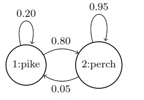
Suppose a person is ice fishing for perch and pike, and notes that if they catch a perch, it is 95% likely that the next fish they catch is a perch, whereas if they catch a pike, it is 20% likely the next fish they catch is a pike.^[This is a thinly reskinned version of the classic exercise involving cars and trucks from Ross, S.M.,2014. Introduction to Probability Models. Tenth edition. Academic Press. Exercise 30, page 279.] We’ll treat the sequence of fish types as a random process \(Y = Y_1, Y_2, \ldots\) with values

The sequence \(Y\) forms a Markov chain with transition probabilities

The easiest way to visual a Markov chain with only a few states is as a state transition diagram. In the case of the pike and perch, the transition diagram is as follows.

State diagram for finite Markov chain generating sequences of fishes. The last fish observed determines the current state and the arrows indicate transition probabilities to the next fish observed.

Like all such transition graphs, the probabilities on the edges going out of a node must sum to one.

Let’s simulate some fishing. The approach is to generate the type of each fish in the sequence, then report the overall proportion of pike.^[With some sleight of hand here for compatibility with Bernoulli variates and to facilitate computing proportions, we have recoded perch as having value 0 rather than 2.] We will start with a random fish drawn according to \(\mbox{bernoulli(1/2)}\).

import numpy as np

T = 100 # number of time points
y = np.zeros(T, dtype=int) # initialize array of outcomes
y[0] = np.random.binomial(1, 0.5) # generate first outcome

for t in range(1, T):
    p = 0.2 if y[t-1] == 1 else 0.05 # determine success probability
    y[t] = np.random.binomial(1, p) # generate outcome

prop = np.mean(y) # calculate proportion of 1's
print(f"Simulated proportion of 1's: {prop:.2f}")

Simulated proportion of 1's: 0.08

Now let’s assume the fish are really running, and run a few simulated chains until \(T = 10,000\).

import numpy as np

np.random.seed(1234)
T = 10000
M = 5
for k in range(M):
    y = np.zeros(T, dtype=int)
    y[0] = np.random.binomial(1, 0.5)
    for t in range(1, T):
        p = 0.2 if y[t-1] == 1 else 0.05
        y[t] = np.random.binomial(1, p)
    prop = np.mean(y)
    print(f"Simulated proportion of 1's: {prop:.3f}")

Simulated proportion of 1's: 0.058
Simulated proportion of 1's: 0.063
Simulated proportion of 1's: 0.060
Simulated proportion of 1's: 0.058
Simulated proportion of 1's: 0.060

The proportion of pike is roughly 0.06.

Ehrenfest’s Urns

Suppose we have two urns, with a total of \(N\) balls distributed between them. At each time step, a ball is chosen uniformly at random from among the balls in both urns and moved to the other urn.^[This model was originally introduced as an example of entropy and equilibrium in P. Ehrenfest and T. Ehrenfest. 1906. Über eine Aufgabe aus der Wahrscheinlichkeitsrechnung, die mit der kinetischen Deutung der Entropievermehrung zusammenhängt. Mathematisch-Naturwissenschaftliche Blätter No. 11 and 12.]

The process defines a Markov chain \(Y\) where transitions are governed by

\(p_{Y_{t+1} \mid Y_t}(y_{t+1} \mid y_t)\) \(= \begin{cases} \displaystyle \frac{y_t}{N} & \mbox{if } \ y_{t + 1} = y_t - 1, \ \mbox{and} \\[6pt] \displaystyle 1 - \frac{y_t}{N} & \mbox{if } \ y_{t + 1} = y_t + 1. \end{cases}\)

The transition probabilities make sure that the value of \(Y_t\) remains between 0 and \(N\). For example,

because \(1 - \frac{y_t}{N} = 1\). Similarly, if \(Y_t = N\), then \(Y_{t+1} = N - 1\).

What happens to the distribution of \(Y_t\) long term? It’s easy to compute by simulation of a single long chain:^[We’ve used a function borrowed from R here called table, defined by \(\mbox{table}(y, A, B)[n] = \sum_{t=1}^T \mbox{I}[y_t = n]\) for \(n \in A:B\). For example, if \(y = (0, 1, 2, 1, 1, 3, 2, 2, 1),\) then \(\mbox{table}(y, 0, 4) = (1, 4, 3, 1, 0),\) because there is one 0, four 1s, three 2s, a single 3, and no 4s among the values of \(y\).]

import numpy as np

N = 100 # population size
T = 1000 # number of time points
y = np.zeros(T, dtype=int) # initialize array of counts
z = np.zeros(T, dtype=int) # initialize array of outcomes
y[0] = N // 2 # set initial count to N/2

for t in range(1, T):
    z[t] = np.random.binomial(1, y[t-1]/N) # generate outcome
    y[t] = y[t-1] - 1 if z[t] else y[t-1] + 1 # update count

p_Y_t_hat = np.bincount(y, minlength=N+1) / T # calculate proportion of counts

Let’s run that with \(N = 10\) and \(T = 100,000\) and display the results as a bar plot.

Long-term distribution of number of balls in the first urn of the Ehrenfest model in which \(N\) balls are distributed between two urns, then at each time step, a ball is chosen uniformly at random move to the other urn. The simulation is based on total of \(T = 100,000\) steps with \(N = 10\) balls, starting with 5 balls in the first urn. The points on the top of the bars are positioned at the mass defined by the binomial distribution, \(\\mbox{binomial}(Y_t \\mid 10, 0.5)\).

import numpy as np
import pandas as pd
import matplotlib.pyplot as plt
from scipy.stats import binom
from plotnine import *

np.random.seed(1234)
N = 10
T = 100000
y = np.zeros(T)
y[0] = 5

for t in range(1, T):
    z_t = np.random.binomial(1, y[t-1]/N)
    y[t] = y[t-1] - z_t + (1 - z_t)

ehrenfest_df = pd.DataFrame({'x': np.arange(1, T+1), 'y': y})

ehrenfest_plot = (
    ggplot(data=ehrenfest_df, mapping=aes(x='y')) +
    geom_bar(color='black', fill='#ffffe8', size=0.2) +
    geom_point(data=pd.DataFrame({'x': np.arange(11), 'y': T * binom.pmf(np.arange(11), 10, 0.5)}),
               mapping=aes(x='x', y='y'), size=3, alpha=0.5) +
    scale_x_continuous(breaks=[0, 2, 4, 6, 8, 10]) +
    scale_y_continuous(breaks=np.arange(0, 300000, 50000), labels=[str(x) for x in np.arange(0, 0.6, 0.1)]) +
    xlab('Y[t]') +
    ylab('proportion')
)

print(ehrenfest_plot)

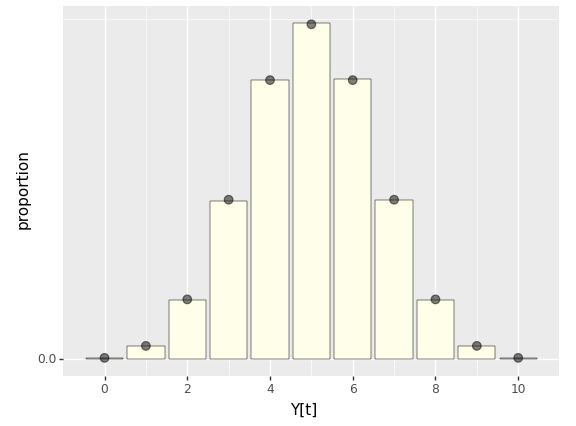
The distribution of \(Y_t\) values is the binomial distribution, as shown by the agreement between the points (the binomial probability mass function) and the bars (the empirical proportion \(Y_t\) spent in each state).^[In the Markov chain Monte Carlo chapter later in the book, we will see how to construct a Markov chain whose long-term frequency distribution matches any given target distribution.]

Page Rank and the random surfer

Pagerank,^[Page, L., Brin, S., Motwani, R. and Winograd, T., 1999. The PageRank citation ranking: Bringing order to the web. Stanford InfoLab Technical Report. Section 2.5 Random Surfer Model.] the innovation behind the original Google search engine ranking system, can be modeled in terms of a random web surfer whose behavior determines a Markov chain. The web is modeled as a set of pages, each of which has a set of outgoing links to other pages. When viewing a particular page, our random surfer chooses the next page to visit by

• if the current page has outgoing links, then with probability \(\lambda\), choose the next page uniformly at random among the outgoing links,

• otherwise (with probability \(1 - \lambda\)), choose the next page to visit uniformly at random among all web pages.

Translating this into the language of random variables, let \(Y = Y_1, Y_2, \ldots\) be the sequence of web pages visited. Our goal now is to define the transition function probabilistically so that we may simulate the random surfer. Let \(L_i \subseteq 1:N\) be the set of outgoing links from page \(i\); each page may have any number of outgoing links from \(0\) to \(N\).

The process \(Y\) is most easily described in terms of an auxiliary process \(Z = Z_1, Z_2, \ldots\) where \(Z_t\) represents

the decision whether to jump to a link from the current page. We define \(Z\) by setting \(Z_t = 0\) if the page \(Y_t\) has no outgoing links, and otherwise setting

If \(Z_t = 1\), we can generate \(Y_{t+1}\) uniformly from the links \(L_{Y_t}\) from page \(Y_t\),

If \(Z_t = 0\), we simply choose a web page uniformly at random from among all \(N\) pages,

This sequence is easy to simulate with L[n] denoting the outgoing links from page n. We start from a page y[1] chosen uniformly at random among all the pages. Then we just simulate subsequent pages according to the process described above.

import numpy as np

# Define L and lambda
L = {1: [2, 3, 4], 2: [4], 3: [4], 4: []}
lam = 0.85

# Set initial values
N = 4
T = 10
y = np.zeros(T, dtype=int)
z = np.zeros(T, dtype=int)

# Set initial value for y
y[0] = np.random.randint(1, N+1)

# Simulate y and z
for t in range(1, T):
    last_page = y[t - 1]
    out_links = L[last_page]
    z[t] = 0 if not out_links else np.random.binomial(1, lam)
    y[t] = np.random.choice(out_links) if z[t] else np.random.randint(1, N+1)
    
print(y)

[4 1 4 2 4 1 4 1 2 4]

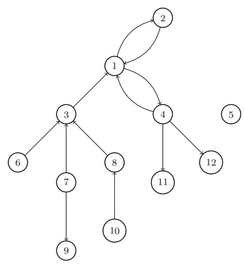
Suppose we have the following graph. A simplified web. Each node represents a web page and each edge is a directed link from one page to another web page.

We can simulate \(T = 100,000\) page visits using the algorithm shown above and display the proportion of time spent on each page.

Proportion of time spent on each page by a random surfer taking \(T = 100,000\) page views starting from a random page with a web structured as in the previous diagram.

import numpy as np
import pandas as pd
import matplotlib.pyplot as plt
import seaborn as sns
from scipy.stats import bernoulli

L = np.zeros((12, 12))
L[[0, 2], [1, 3]] = 1
L[1, 0] = 1
L[2, 0] = 1
L[[3, 10, 11], [0, 9, 10]] = 1
L[4, :] = 1
L[5, 2] = 1
L[[6, 8], [2, 8]] = 1
L[7, 2] = 1
L[8, :] = 1
L[9, 7] = 1
L[10, :] = 1
L[11, :] = 1

lmbda = 0.90
theta = np.zeros((12, 12))
for i in range(12):
    if np.sum(L[i, :]) == 0:
        theta[i, :] = np.repeat(1/12, 12)
    else:
        theta[i, :] = lmbda * L[i, :] / np.sum(L[i, :]) + \
                      (1 - lmbda) * np.repeat(1/12, 12)

np.random.seed(1234)
T = int(1e5)
y = np.zeros(T, dtype=int)
y[0] = np.random.choice(12, 1)[0]
for t in range(1, T):
    y[t] = np.random.choice(12, 1, p=theta[y[t-1], :])[0]

visited = np.bincount(y)

pagerank_df = pd.DataFrame({'x': range(1, T+1), 'y': y})

pagerank_plot = (sns
                 .catplot(x='y', data=pagerank_df, kind='count', color='#ffffe8', edgecolor='black', linewidth=0.2)
                 .set(xlabel='page', ylabel='rank (proportion of time on page)', 
                      xticks=np.arange(12), yticks=[0, 0.1*T, 0.2*T, 0.3*T], yticklabels=[0, 0.1, 0.2, 0.3])
                 .fig
                )
sns.despine()

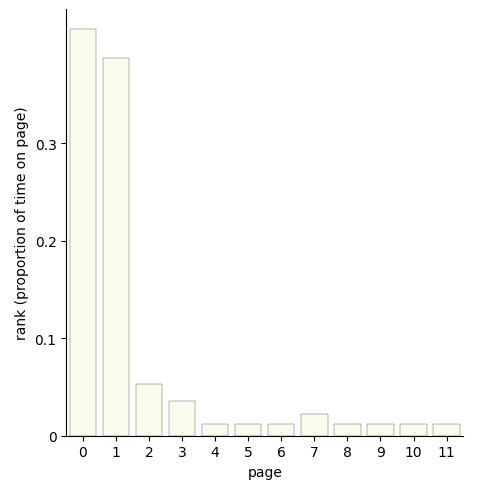
Page 1 is the most central hub. Pages 5, 6, 7, and 10 have no links coming into them and can only be visited by random chance, so all should have the same chance of being visited by the random surfer. Pages 11 and 12 are symmetric, and indeed have the same probability. There is a slight difference between the views of page 9 and 10 in that it possible to get to 9 from 7, but 10 is only visited by chance.

For a Markox transition matrix, the limiting probabilities of being in a certain state as \(n \rightarrow \infty\) are given by the solution to the following set of linear equations. \(p_j^* = \sum_{i=1}^{\infty} p_i^* p_{ij}\)

1. A number from \(1\) to \(m\) is chosen at random, at each of the times \(t = 1, 2, . . .\). A system is said to be in the state \(e_{0}\), if no number has yet been chosen, and in the state \(e_{i}\), if the largest number so far chosen is \(i\). Show that the random process described by this model is a Markov chain. Find the corresponding transition probabilities \(p_{ij} (i, j= 0, 1 , . . . , m)\).

Solution

Since state \(i\) signifies that the highest number chosen so far is \(i\),
what is the probability the next number is lower than \(i\) and you stay in state \(i\)? Well, there are \(m\) possible numbers that could get picked and \(i\) of them are less than or equal to \(i\) giving:
\(p_{ii} = \frac{i}{m}\)
What now if we’re in \(i\) and we want to know what the probability of being in state \(j\) is next.
Well, if \(j<i\) then it’s zero because you can’t go to a lower number in this game.
If, however, \(j\) is not lower then there are \(m\) possible numbers that could get called and only one of them is \(j\), giving:
\(p_{ij} = \frac{1}{m}, j>i\)
\(p_{ij} = 0, j<i\)

Solution

To show that the random process described by this model is a Markov chain, we need to demonstrate that the future state of the process depends only on the current state and not on any of the past states. In this case, the current state is determined by the largest number chosen so far, and the future state is determined by the next number that is chosen.
Formally, we can say that the Markov property holds if:
\(P\left(X_{t+1}=j|X_{t}=i,X_{t-1}=i_{t-1},...,X_{1}=i_{1}\right)= P\left(X_{t+1}=j∣X_{t}=i\right)\)
where \(X_t\) denotes the state of the system at time \(t\), and \(P(X_{t+1}=j | X_t=i)\) represents the probability of transitioning from state \(i\) to state \(j\).
In this case, since the future state depends only on the largest number chosen so far (i.e., the current state) and the next number that is chosen, we can say that the Markov property holds.
The transition probabilities can be calculated as follows:
Let \(p_i\) be the probability that the largest number chosen so far is \(i\).
Then, at any given time \(t\), the probability of choosing a number greater than \(i\) is \((m-i)/m\), and the probability of choosing a number less than or equal to \(i\) is \(i/m\).
Therefore, we can write the transition probabilities as:
\(p_{e_0,e_1} = \frac{1}{m}\)
\(p_{e_i,e_{i+1}} = \frac{m-i}{m}\), for \(i = 0,1,...,m-1\)
\(p_{e_i,e_j} = \frac{i}{m}\), for \(j \le i, i = 1,...,m\)
\(p_{e_i,e_0}= 1 - p_{e_i,e_{i+1}} - \sum_{j=1}^{i}p_{e_i,e_j}\), where the sum is taken over all \(j \le i, i = 1,...,m\)
Note that \(p_{e_i,e_0}\) represents the probability of starting over (i.e., going back to the state \(e_0\)) after reaching state \(e_i\).
These transition probabilities satisfy the Markov property, and therefore, the random process described by this model is a Markov chain.

2. In the preceding problem, which states are persistent and which transient?

Solution

Since state \(i\) signifies that the highest number chosen so far is \(i\),
what is the probability the next number is lower than \(i\) and you stay in state \(i\)? Well, there are \(m\) possible numbers that could get picked and \(i\) of them are less than or equal to \(i\) giving:
\(p_{ii} = \frac{i}{m}\)
What now if we’re in \(i\) and we want to know what the probability of being in state \(j\) is next.
Well, if \(j<i\) then it’s zero because you can’t go to a lower number in this game.
If, however, \(j\) is not lower then there are \(m\) possible numbers that could get called and only one of them is \(j\), giving:
\(p_{ij} = \frac{1}{m}, j>i\)
\(p_{ij} = 0, j<i\)

Solution

In this model, the state \(e_0\) (no number has been chosen yet) is a transient state because once a number is chosen, the system moves to one of the other states.
All the other states, \(e_1\) through \(e_m\), are persistent states because once the system reaches any of these states, it will never return to the state \(e_0\) (no number has been chosen yet). This is because a number has already been chosen, and the largest number chosen so far is at least \(1\).
Therefore, the system will always remain in one of the persistent states, and will never return to the state \(e_0\).

3. Suppose \(m = 4\) in Problem \(1\). Find the matrix \(P(2) = \|p_{i,j}(2)\)||, where \(p_{i,j}(2)\) is the probability that the system will go from state \(e_i\), to state \(e_j\), in \(2\) steps.

Solution

To do this properly we need to first construct the matrix \(P\).
\(P = \left( \begin{array}{ccccc} 0 & \frac{1}{4} & \frac{1}{4} & \frac{1}{4} & \frac{1}{4} \\ 0 & \frac{1}{4} & \frac{1}{4} & \frac{1}{4} & \frac{1}{4} \\ 0 & 0 & \frac{1}{2} & \frac{1}{4} & \frac{1}{4} \\ 0 & 0 & 0 & \frac{3}{4} & \frac{1}{4} \\ 0 & 0 & 0 & 0 & 1 \end{array} \right)\)
Then we square it:
\(P^2 = \left( \begin{array}{ccccc} 0 & \frac{1}{16} & \frac{3}{16} & \frac{5}{16} & \frac{7}{16} \\ 0 & \frac{1}{16} & \frac{3}{16} & \frac{5}{16} & \frac{7}{16} \\ 0 & 0 & \frac{1}{4} & \frac{5}{16} & \frac{7}{16} \\ 0 & 0 & 0 & \frac{9}{16} & \frac{7}{16} \\ 0 & 0 & 0 & 0 & 1 \end{array} \right)\)

4. An urn contains a total of N balls, some black and some white. Samples are drawn from the urn, \(m\) balls at a time \((m < N)\). After drawing each sample,the black balls are returned to the urn, while the white balls are replaced by black balls and then returned to the urn. If the number of white balls in the um is \(i\), we say that the “system” is in the state \(e\);. Prove that the random process described by this model is a Markov chain (imagine that samples are drawn at the times \(t = 1, 2,\ldots\) and that the system has some initial probability distribu­tion). Find the corresponding transition probabilities \(P_{i,j} (i,j = 0, 1 ,\ldots, N)\).Which states are persistent and which transient?

Solution

So, if we start with \(i\) balls in the urn, what is the probability that we have \(j\) after drawing \(m\) and discarding all the white balls.
The obvious first simplification we can make is that you can’t end up with fewer that the \(N-m\) white balls after drawing:
\(p_{ij} = 0, j > N - m\)
You also can’t gain white balls
\(p_{ij} = 0, j > i\)
OK! now for the interesting one.
There are \(\binom{N}{m}\) ways to draw \(m\) balls from the urn.
In any given step, you are going to draw \(i-j\) white balls from a total of \(i\) and \(m - i +j\) black balls from a total of \(N-i\).
Thus there are \(\binom{i}{i-j}\binom{N-i}{m - i +j}\) ways to make that draw, \(p_{ij} = \frac{\binom{i}{i-j}\binom{N-i}{m - i +j}}{\binom{N}{m}}, \text{otherwise}\).

5. In the preceding problems, let \(N = 8, m =4,\) and suppose there are initially \(5\) white balls in the urn. What is the probability that no white balls are left after \(2\) .drawings (of \(4\) balls each)?

Solution

Once again, we start building the transition matrix.
\(P = \left( \begin{array}{ccccccccc} 1 & 0 & 0 & 0 & 0 & 0 & 0 & 0 & 0 \\ \frac{1}{2} & \frac{1}{2} & 0 & 0 & 0 & 0 & 0 & 0 & 0 \\ \frac{3}{14} & \frac{4}{7} & \frac{3}{14} & 0 & 0 & 0 & 0 & 0 & 0 \\ \frac{1}{14} & \frac{3}{7} & \frac{3}{7} & \frac{1}{14} & 0 & 0 & 0 & 0 & 0 \\ \frac{1}{70} & \frac{8}{35} & \frac{18}{35} & \frac{8}{35} & \frac{1}{70} & 0 & 0 & 0 & 0 \\ 0 & \frac{1}{14} & \frac{3}{7} & \frac{3}{7} & \frac{1}{14} & 0 & 0 & 0 & 0 \\ 0 & 0 & \frac{3}{14} & \frac{4}{7} & \frac{3}{14} & 0 & 0 & 0 & 0 \\ 0 & 0 & 0 & \frac{1}{2} & \frac{1}{2} & 0 & 0 & 0 & 0 \\ 0 & 0 & 0 & 0 & 1 & 0 & 0 & 0 & 0 \end{array} \right)\)

And then just square it!

\(P^2 = \left( \begin{array}{ccccccccc} 1 & 0 & 0 & 0 & 0 & 0 & 0 & 0 & 0 \\ \frac{3}{4} & \frac{1}{4} & 0 & 0 & 0 & 0 & 0 & 0 & 0 \\ \frac{107}{196} & \frac{20}{49} & \frac{9}{196} & 0 & 0 & 0 & 0 & 0 & 0 \\ \frac{75}{196} & \frac{24}{49} & \frac{6}{49} & \frac{1}{196} & 0 & 0 & 0 & 0 & 0 \\ \frac{1251}{4900} & \frac{624}{1225} & \frac{264}{1225} & \frac{24}{1225} & \frac{1}{4900} & 0 & 0 & 0 & 0 \\ \frac{39}{245} & \frac{471}{980} & \frac{153}{490} & \frac{23}{490} & \frac{1}{980} & 0 & 0 & 0 & 0 \\ \frac{22}{245} & \frac{102}{245} & \frac{393}{980} & \frac{22}{245} & \frac{3}{980} & 0 & 0 & 0 & 0 \\ \frac{3}{70} & \frac{23}{70} & \frac{33}{70} & \frac{3}{20} & \frac{1}{140} & 0 & 0 & 0 & 0 \\ \frac{1}{70} & \frac{8}{35} & \frac{18}{35} & \frac{8}{35} & \frac{1}{70} & 0 & 0 & 0 & 0 \end{array} \right)\)

Telling us there is a \(39\) in \(245\) chance that if we start with \(5\) balls that we’ll be at zero after two steps.

Key Points