Introduction
Overview
Teaching: 5 min
Exercises: 0 minQuestions
What sort of scientific questions can we answer with image processing / computer vision?
What are morphometric problems?
What are colorimetric problems?
Objectives
Recognize scientific questions that could be solved with image processing / computer vision.
Recognize morphometric problems (those dealing with the number, size, or shape of the objects in an image).
Recognize colorimetric problems (those dealing with the analysis of the color or the objects in an image).
We can use relatively simple image processing and computer vision techniques in Python, using the skimage library. With careful experimental design, a digital camera or a flatbed scanner, in conjunction with some Python code, can be a powerful instrument in answering many different kinds of problems. Consider the following two types of problems that might be of interest to a scientist.
Morphometrics
Morphometrics involves counting the number of objects in an image, analyzing the size of the objects, or analyzing the shape of the objects. For example, we might be interested automatically counting the number of bacterial colonies growing in a Petri dish, as shown in this image:
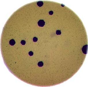
We could use image processing to find the colonies, count them, and then highlight their locations on the original image, resulting in an image like this:

Colorimetrics
Colorimetrics involves analyzing the color of objects in an image. For example, consider this video of a titrant being added to an analyte (click on the image to see the video):
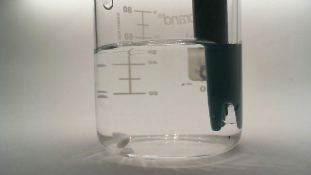
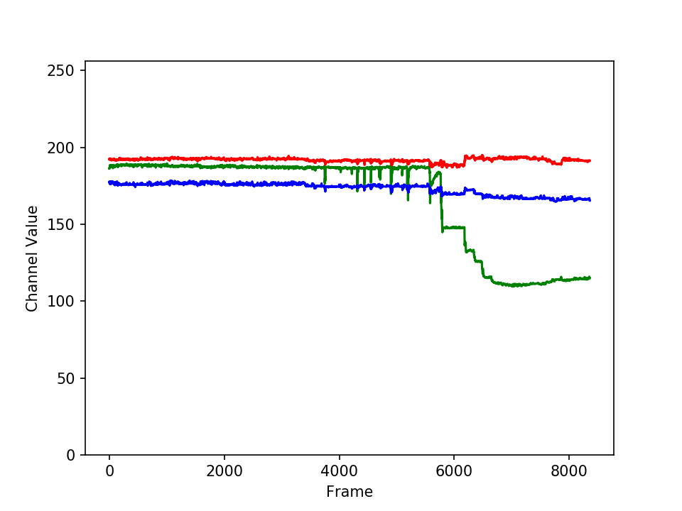
We could use image processing to look at the color of the solution, and determine when the titration is complete. This graph shows how the three component colors (red, green, and blue) of the solution change over time; the change in the solution’s color is obvious.
Why write a program to do that?
Note that you can easily manually count the number of bacteria colonies shown in the morphometric example above. Why should we learn how to write a Python program to do a task we could easily perform with our own eyes? There are at least two reasons to learn how to perform tasks like these with Python and skimage:
What if there are many more bacteria colonies in the Petri dish? For example, suppose the image looked like this:
Manually counting the colonies in that image would present more of a challenge. A Python program using skimage could count the number of colonies more accurately, and much more quickly, than a human could.
What if you have hundreds, or thousands, of images to consider? Imagine having to manually count colonies on several thousand images like those above. A Python program using skimage could move through all of the images in seconds; how long would a graduate student require to do the task? Which process would be more accurate and repeatable?
As you can see, the simple image processing / computer vision techniques you will learn during this workshop can be very valuable tools for scientific research.
As we move through this workshop, we will return to these sample problems several times, and you will solve each of these problems during the end-of-workshop challenges.
Let’s get started, by learning some basics about how images are represented and stored digitally.
Key Points
Simple Python and skimage (scikit-image) techniques can be used to solve genuine morphometric and colorimetric problems.
Morphometric problems involve the number, shape, and / or size of the objects in an image.
Colorimetric problems involve analyzing the color of the objects in an image.
Image Basics
Overview
Teaching: 35 min
Exercises: 15 minQuestions
How are images represented in digital format?
Objectives
Define the terms bit, byte, kilobyte, megabyte, etc.
Explain how a digital image is composed of pixels.
Explain the left-hand coordinate system used in digital images.
Explain the RGB additive color model used in digital images.
Explain the characteristics of the BMP, JPEG, and TIFF image formats.
Explain the difference between lossy and lossless compression.
Explain the advantages and disadvantages of compressed image formats.
Explain what information could be contained in image metadata.
The images we see on hard copy, view with our electronic devices, or process with our programs are represented and stored in the computer as numeric abstractions, approximations of what we see with our eyes in the real world. Before we begin to learn how to process images with Python programs, we need to spend some time understanding how these abstractions work.
Bits and bytes
Before we talk specifically about images, we first need to understand how numbers are stored in a modern digital computer. When we think of a number, we do so using a decimal, or base-10 place-value number system. For example, a number like 659 is 6 × 10² + 5 × 101 + 9 × 100. Each digit in the number is multiplied by a power of 10, based on where it occurs, and there are 10 digits that can occur in each position (0, 1, 2, 3, 4, 5, 6, 7, 8, 9).
In principle, computers could be constructed to represent numbers in exactly the same way. But, as it turns out, the electronic circuits inside a computer are much easier to construct if we restrict the numeric base to only two, versus 10. (It is easier for circuitry to tell the difference between two voltage levels than it is to differentiate between 10 levels.) So, values in a computer are stored using a binary, or base-2 place-value number system.
In this system, each symbol in a number is called a bit instead of a digit, and there are only two values for each bit (0 and 1). We might imagine a four-bit binary number, 1101. Using the same kind of place-value expansion as we did above for 659, we see that 1101 = 1 × 23 + 1 × 22 + 0 × 21 + 1 × 20, which if we do the math is 8 + 4 + 0 + 1, or 13 in decimal.
Internally, computers have a minimum number of bits that they work with at a given time: eight. A group of eight bits is called a byte. The amount of memory (RAM) and drive space our computers have is quantified by terms like Megabytes (MB), Gigabytes (GB), and Terabytes (TB). The following table provides more formal definitions for these terms.
| Unit | Abbreviation | Size |
|---|---|---|
| Kilobyte | KB | 1024 bytes |
| Megabyte | MB | 1024 KB |
| Gigabyte | GB | 1024 MB |
| Terabyte | TB | 1024 GB |
Pixels
It is important to realize that images are stored as rectangular arrays of hundreds, thousands, or millions of discrete “picture elements,” otherwise known as pixels. Each pixel can be thought of as a single square point of colored light.
For example, consider this image of a maize seedling, with a square area designated by a red box:
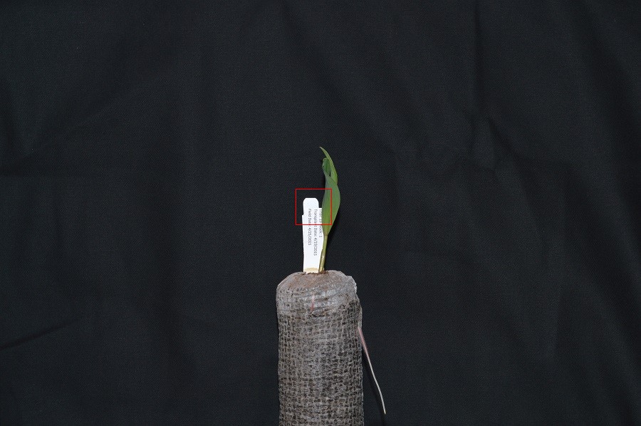
Now, if we zoomed in close enough to see the pixels in the red box, we would see something like this:
Note that each square in the enlarged image area – each pixel – is all one color, but that each pixel can have a different color from its neighbors. Viewed from a distance, these pixels seem to blend together to form the image we see.
Coordinate system
When we process images, we can access, examine, and / or change the color of any pixel we wish. To do this, we need some convention on how to access pixels individually; a way to give each one a name, or an address of a sort.
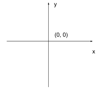
The most common manner to do this, and the one we will use in our programs, is to assign a modified Cartesian coordinate system to the image. The coordinate system we usually see in mathematics has a horizontal x-axis and a vertical y-axis, like this:
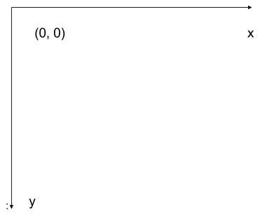
The modified coordinate system used for our images will have only positive coordinates, the origin will be in the upper left corner instead of the center, and y coordinate values will get larger as they go down instead of up, like this:
This is called a left-hand coordinate system. If you hold your left hand in front of your face and point your thumb at the floor, your extended index finger will correspond to the x-axis while your thumb represents the y-axis.
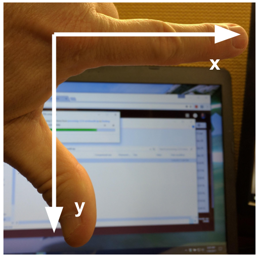
Until you have worked with images for a while, the most common mistake that you will make with coordinates is to forget that y coordinates get larger as they go down instead of up as in a normal Cartesian coordinate system.
Color model
Digital images use some color model to create a broad range of colors from a small set of primary colors. Although there are several different color models that are used for images, the most commonly occurring one is the RGB (Red, Green, Blue) model.
The RGB model is an additive color model, which means that the primary colors are mixed together to form other colors. In the RGB model, the primary colors are red, green, and blue – thus the name of the model. Each primary color is often called a channel.
Most frequently, the amount of the primary color added is represented as an integer in the closed range [0, 255]. Therefore, there are 256 discrete amounts of each primary color that can be added to produce another color. The number of discrete amounts of each color, 256, corresponds to the number of bits used to hold the color channel value, which is eight (28=256). Since we have three channels, this is called 24-bit color depth.
Any particular color in the RGB model can be expressed by a triplet of integers in [0, 255], representing the red, green, and blue channels, respectively. A larger number in a channel means that more of that primary color is present.
Thinking about RGB colors (3 min)
Suppose that we represent colors as triples (r, g, b), where each of r, g, and b is an integer in [0, 255]. What colors are represented by each of these triples? (Try to answer these questions without reading further.)
- (255, 0, 0)
- (0, 255, 0)
- (0, 0, 255)
- (255, 255, 255)
- (0, 0, 0)
- (128, 128, 128)
Solution
- (255, 0, 0) represents red, because the red channel is maximized, while the other two channels have the minimum values.
- (0, 255, 0) represents green.
- (0, 0, 255) represents blue.
- (255, 255, 255) is a little harder. When we mix the maximum value of all three color channels, we see the color white.
- (0, 0, 0) represents the absence of all color, or black.
- (128, 128, 128) represents a medium shade of gray. Note that the 24-bit RGB color model provides at least 254 shades of gray, rather than only fifty.
Note that the RGB color model may run contrary to your experience, especially if you have mixed primary colors of paint to create new colors. In the RGB model, the lack of any color is black, while the maximum amount of each of the primary colors is white. With physical paint, we might start with a white base, and then add differing amounts of other paints to produce a darker shade.
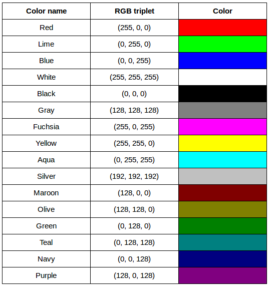
After completing the previous challenge, we can look at some further examples of 24-bit RGB colors, in a visual way. The image in the next challenge shows some color names, their 24-bit RGB triplet values, and the color itself.
RGB color table (4 min)
We cannot really provide a complete table. To see why, answer this question: How many possible colors can be represented with the 24-bit RGB model?
Solution
There are 24 total bits in an RGB color of this type, and each bit can be on or off, and so there are 224 = 16,777,216 possible colors with our additive, 24-bit RGB color model.
Although 24-bit color depth is common, there are other options. We might have 8-bit color (3 bits for red and green, but only 2 for blue, providing 8 × 8 × 4 = 256 colors) or 16-bit color (4 bits for red, green, and blue, plus 4 more for transparency, providing 16 × 16 × 16 = 4096 colors), for example. There are color depths with more than eight bits per channel, but as the human eye can only discern approximately 10 million different colors, these are not often used.
If you are using an older or inexpensive laptop screen or LCD monitor to view images, it may only support 18-bit color, capable of displaying 64 × 64 × 64 = 262,144 colors. 24-bit color images will be converted in some manner to 18-bit, and thus the color quality you see will not match what is actually in the image.
We can combine our coordinate system with the 24-bit RGB color model to gain a conceptual understanding of the images we will be working with. An image is a rectangular array of pixels, each with its own coordinate. Each pixel in the image is a square point of colored light, where the color is specified by a 24-bit RGB triplet. Such an image is an example of raster graphics.
Image formats
Although the images we will manipulate in our programs are conceptualized as rectangular arrays of RGB triplets, they are not necessarily created, stored, or transmitted in that format. There are several image formats we might encounter, and we should know the basics of at least of few of them. Some formats we might encounter, and their file extensions, are shown in this table:
| Format | Extension |
|---|---|
| Device-Independent Bitmap (BMP) | .bmp |
| Joint Photographic Experts Group (JPEG) | .jpg or .jpeg |
| Tagged Image File Format (TIFF) | .tif or .tiff |
BMP
The file format that comes closest to our preceding conceptualization of images is the Device-Independent Bitmap, or BMP, file format. BMP files store raster graphics images as long sequences of binary-encoded numbers that specify the color of each pixel in the image. Since computer files are one-dimensional structures, the pixel colors are stored one row at a time. That is, the first row of pixels (those with y-coordinate 0) are stored first, followed by the second row (those with y-coordinate 1), and so on. Depending on how it was created, a BMP image might have 8-bit, 16-bit, or 24-bit color depth.
24-bit BMP images have a relatively simple file format, can be viewed and loaded across a wide variety of operating systems, and have high quality. However, BMP images are not compressed, resulting in very large file sizes for any useful image resolutions.
The idea of image compression is important to us for two reasons: first, compressed images have smaller file sizes, and are therefore easier to store and transmit; and second, compressed images may not have as much detail as their uncompressed counterparts, and so our programs may not be able to detect some important aspect if we are working with compressed images. Since compression is important to us, we should take a brief detour and discuss the concept.
Image compression
Let’s begin our discussion of compression with a simple challenge.
BMP image size (8 min)
Imagine that we have a fairly large, but very boring image: a 5,000 × 5,000 pixel image composed of nothing but white pixels. If we used an uncompressed image format such as BMP, with the 24-bit RGB color model, how much storage would be required for the file?
Solution
In such an image, there are 5,000 × 5,000 = 25,000,000 pixels, and 24 bits for each pixel, leading to 25,000,000 × 24 = 600,000,000 bits, or 75,000,000 bytes (71.5MB). That is quite a lot of space for a very uninteresting image!
Since image files can be very large, various compression schemes exist for saving (approximately) the same information while using less space. These compression techniques can be categorized as lossless or lossy.
Lossless compression
In lossless image compression, we apply some algorithm (i.e., a computerized procedure) to the image, resulting in a file that is significantly smaller than the uncompressed BMP file equivalent would be. Then, when we wish to load and view or process the image, our program reads the compressed file, and reverses the compression process, resulting in an image that is identical to the original. Nothing is lost in the process – hence the term “lossless.”
The general idea of lossless compression is to somehow detect long patterns of bytes in a file that are repeated over and over, and then assign a smaller bit pattern to represent the longer sample. Then, the compressed file is made up of the smaller patterns, rather than the larger ones, thus reducing the number of bytes required to save the file. The compressed file also contains a table of the substituted patterns and the originals, so when the file is decompressed it can be made identical to the original before compression.
To provide you with a concrete example, consider the 71.5 MB white BMP image discussed above. When put through the zip compression utility on Microsoft Windows, the resulting .zip file is only 72 KB in size! That is, the .zip version of the image is three orders of magnitude smaller than the original, and it can be decompressed into a file that is byte-for-byte the same as the original. Since the original is so repetitious – simply the same color triplet repeated 25,000,000 times – the compression algorithm can dramatically reduce the size of the file.
If you work with .zip or .gz archives, you are dealing with lossless compression.
Lossy compression
Lossy compression takes the original image and discards some of the detail in it, resulting in a smaller file format. The goal is to only throw away detail that someone viewing the image would not notice. Many lossy compression schemes have adjustable levels of compression, so that the image creator can choose the amount of detail that is lost. The more detail that is sacrificed, the smaller the image files will be – but of course, the detail and richness of the image will be lower as well.
This is probably fine for images that are shown on Web pages or printed off on 4 × 6 photo paper, but may or may not be fine for scientific work. You will have to decide whether the loss of image quality and detail are important to your work, versus the space savings afforded by a lossy compression format.
It is important to understand that once an image is saved in a lossy compression format, the lost detail is just that – lost. I.e., unlike lossless formats, given an image saved in a lossy format, there is no way to reconstruct the original image in a byte-by-byte manner.
JPEG
JPEG images are perhaps the most commonly encountered digital images today. JPEG uses lossy compression, and the degree of compression can be tuned to your liking. It supports 24-bit color depth, and since the format is so widely used, JPEG images can be viewed and manipulated easily on all computing platforms.
Examining actual image sizes (5 min)
Let us see the effects of image compression on image size with actual images. Open a terminal and navigate to the Desktop/workshops/image-processing/02-image-basics directory. This directory contains a simple program, ws.py that creates a square white image of a specified size, and then saves it as a BMP and as a JPEG image.
To create a 5,000 x 5,000 white square, execute the program by typing python ws.py 5000 and then hitting enter. Then, examine the file sizes of the two output files, ws.bmp and ws.jpg. Does the BMP image size match our previous prediction? How about the JPEG?
Solution
The BMP file, ws.bmp, is 75,000,054 bytes, which matches our prediction very nicely. The JPEG file, ws.jpg, is 392,503 bytes, two orders of magnitude smaller than the bitmap version.
Comparing lossless versus lossy compression (8 min)
Let us see a hands-on example of lossless versus lossy compression. Once again, open a terminal and navigate to the Desktop/workshops/image-processing/02-image-basics directory. The two output images, ws.bmp and ws.jpg, should still be in the directory, along with another image, tree.jpg.
We can apply lossless compression to any file by using the zip command. Recall that the ws.bmp file contains 75,000,054 bytes. Apply lossless compression to this image by executing the following command: zip ws.zip ws.bmp. This command tells the computer to create a new compressed file, ws.zip, from the original bitmap image. Execute a similar command on the tree JPEG file: zip tree.zip tree.jpg.
Having created the compressed file, use the ls -al command to display the contents of the directory. How big are the compressed files? How do those compare to the size of ws.bmp and tree.jpg? What can you conclude from the relative sizes?
Solution
Here is a partial directory listing, showing the sizes of the relevant files there:
-rw-rw-r– 1 diva diva 154344 Jun 18 08:32 tree.jpg
-rw-rw-r– 1 diva diva 146049 Jun 18 08:53 tree.zip
-rw-rw-r– 1 diva diva 75000054 Jun 18 08:51 ws.bmp
-rw-rw-r– 1 diva diva 72986 Jun 18 08:53 ws.zip
We can see that the regularity of the bitmap image (remember, it is a 5,000 x 5,000 pixel image containing only white pixels) allows the lossless compression scheme to compress the file quite effectively. On the other hand, compressing tree.jpg does not create a much smaller file; this is because the JPEG image was already in a compressed format.
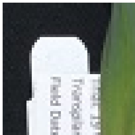
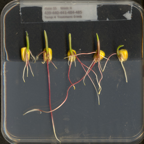
Here is an example showing how JPEG compression might impact image quality. Consider this image of several maize seedlings (scaled down here from 11,339 × 11,336 pixels in order to fit the display).
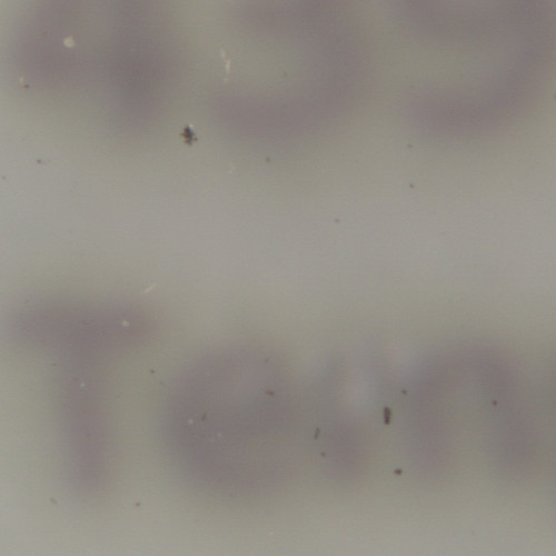
Now, let us zoom in and look at a small section of the label in the original, first in the uncompressed format:
Here is the same area of the image, but in JPEG format. We used a fairly aggressive compression parameter to make the JPEG, in order to illustrate the problems you might encounter with the format.
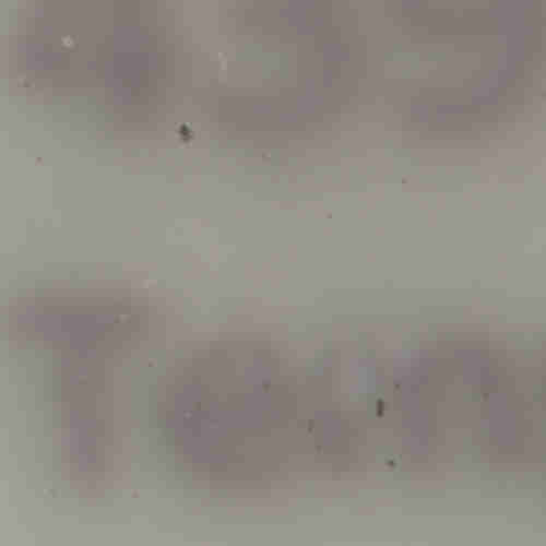
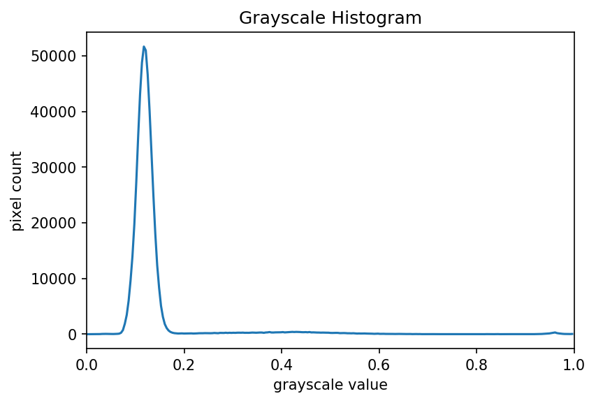
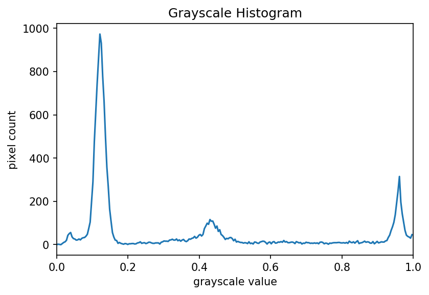
The JPEG image is of clearly inferior quality. It has less color variation and noticeable pixelation. Quality differences become even more marked when one examines the color histograms for each image. A histogram shows how often each color value appears in an image. The histograms for the uncompressed (left) and compressed (right) images are shown below:
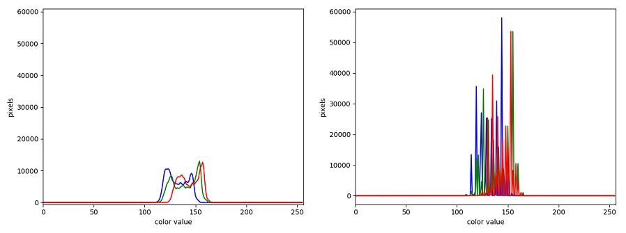
We we learn how to make histograms such as these later on in the workshop. The differences in the color histograms are even more apparent than in the images themselves; clearly the colors in the JPEG image are different from the uncompressed version.
If the quality settings for your JPEG images are high (and the compression rate therefore relatively low), the images may be of sufficient quality for your work. It all depends on how much quality you need, and what restrictions you have on image storage space. Another consideration may be where the images are stored. For example, if your images are stored in the cloud and therefore must be downloaded to your system before you use them, you may wish to use a compressed image format to speed up file transfer time.
TIFF
TIFF images are popular with publishers, graphics designers, and photographers. TIFF images can be uncompressed, or compressed using either lossless or lossy compression schemes, depending on the settings used, and so TIFF images seem to have the benefits of both the BMP and JPEG formats. The main disadvantage of TIFF images (other than the size of images in the uncompressed version of the format) is that they are not universally readable by image viewing and manipulation software.
Metadata
JPEG and TIFF images support the inclusion of metadata in images. Metadata is textual information that is contained within an image file. Metadata holds information about the image itself, such as when the image was captured, where it was captured, what type of camera was used and with what settings, etc. We normally don’t see this metadata when we view an image, but we can access it if we wish. For example, consider this image of a tree flowering in spring:
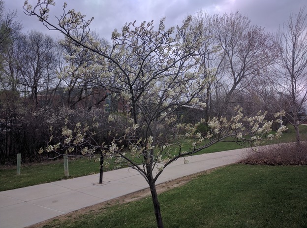
What metadata do you suppose this image contains? One way we can find out is by using ImageMagick, a public domain image processing program that is available for many different computing platforms. ImageMagick is installed on the virtual machine used for this workshop. To display the metadata for an image, we can execute the identify -verbose <file> command from the terminal. If we were to view the tree image metadata with ImageMagick, we would see this information, plus another 100 lines or so:
[Jpeg] Compression Type:	Baseline
[Jpeg] Data Precision:	8 bits
[Jpeg] Image Height:	463 pixels
[Jpeg] Image Width:	624 pixels
[Jpeg] Number of Components:	3
[Jpeg] Component 1:	Y component: Quantization table 0, Sampling factors 2 horiz/2 vert
[Jpeg] Component 2:	Cb component: Quantization table 1, Sampling factors 1 horiz/1 vert
[Jpeg] Component 3:	Cr component: Quantization table 1, Sampling factors 1 horiz/1 vert
[Jfif] Version:	1.1
[Jfif] Resolution Units:	inch
[Jfif] X Resolution:	72 dots
[Jfif] Y Resolution:	72 dots
[Exif SubIFD] Exposure Time:	657/1000000 sec
[Exif SubIFD] F-Number:	F2
[Exif SubIFD] Exposure Program:	Program normal
[Exif SubIFD] ISO Speed Ratings:	40
[Exif SubIFD] Exif Version:	2.20
[Exif SubIFD] Date/Time Original:	2017:04:10 12:04:06
[Exif SubIFD] Date/Time Digitized:	2017:04:10 12:04:06
[Exif SubIFD] Components Configuration:	YCbCr
[Exif SubIFD] Shutter Speed Value:	1/1520 sec
[Exif SubIFD] Aperture Value:	F2
[Exif SubIFD] Brightness Value:	8.89
[Exif SubIFD] Exposure Bias Value:	0 EV
[Exif SubIFD] Max Aperture Value:	F2
[Exif SubIFD] Subject Distance:	0.0 metres
[Exif SubIFD] Metering Mode:	Center weighted average
[Exif SubIFD] Flash:	Flash did not fire, auto
[Exif SubIFD] Focal Length:	3.82 mm
[Exif SubIFD] Sub-Sec Time:	025669
[Exif SubIFD] Sub-Sec Time Original:	025669
[Exif SubIFD] Sub-Sec Time Digitized:	025669
[Exif SubIFD] FlashPix Version:	1.00
[Exif SubIFD] Color Space:	sRGB
[Exif SubIFD] Exif Image Width:	4160 pixels
[Exif SubIFD] Exif Image Height:	3088 pixels
[Exif SubIFD] Sensing Method:	One-chip color area sensor
[Exif SubIFD] Scene Type:	Directly photographed image
[Exif SubIFD] Custom Rendered:	Custom process
[Exif SubIFD] Exposure Mode:	Auto exposure
[Exif SubIFD] White Balance Mode:	Auto white balance
[Exif SubIFD] Scene Capture Type:	Standard
[Exif SubIFD] Contrast:	None
[Exif SubIFD] Saturation:	None
[Exif SubIFD] Sharpness:	None
[Exif SubIFD] Subject Distance Range:	Unknown
[Exif SubIFD] Unknown tag (0xea1c):	[2060 bytes]
[Exif SubIFD] Unknown tag (0xea1d):	4264
[Exif IFD0] Unknown tag (0x0100):	4160
[Exif IFD0] Unknown tag (0x0101):	3088
[Exif IFD0] Image Description:	Flowering tree
[Exif IFD0] Make:	motorola
[Exif IFD0] Model:	Nexus 6
[Exif IFD0] Orientation:	Top, left side (Horizontal / normal)
[Exif IFD0] X Resolution:	72 dots per inch
[Exif IFD0] Y Resolution:	72 dots per inch
[Exif IFD0] Resolution Unit:	Inch
[Exif IFD0] Software:	HDR+ 1.0.126161355r
[Exif IFD0] Date/Time:	2017:04:10 12:04:06
[Exif IFD0] Artist:	Mark M. Meysenburg
[Exif IFD0] YCbCr Positioning:	Center of pixel array
[Exif IFD0] Unknown tag (0x4746):	5
[Exif IFD0] Unknown tag (0x4749):	99
[Exif IFD0] Windows XP Title:	Flowering tree
[Exif IFD0] Windows XP Author:	Mark M. Meysenburg
[Exif IFD0] Windows XP Subject:	Nature
[Exif IFD0] Unknown tag (0xea1c):	[2060 bytes]
[Interoperability] Interoperability Version:	1.00
[GPS] GPS Version ID:	2.200
[GPS] GPS Latitude Ref:	N
[GPS] GPS Latitude:	40.0° 37.0' 19.33999999999571"
[GPS] GPS Longitude Ref:	W
[GPS] GPS Longitude:	-96.0° 56.0' 46.74000000003048"
[GPS] GPS Altitude Ref:	Sea level
[GPS] GPS Altitude:	405 metres
[GPS] GPS Time-Stamp:	17:4:3 UTC
Reviewing the metadata, you can see things like the location where the image was taken, the make and model of the Android smartphone used to capture the image, the date and time when it was captured, and more. Two tags, containing the image description and the “artist,” were added manually. Depending on how you intend to use images, the metadata contained within the images may be important or useful to you. However, care must be taken when using our computer vision library, skimage, to write images. We will examine metadata a little more closely in the skimage Images episode.
Summary of image formats
The following table summarizes the characteristics of the BMP, JPEG, and TIFF image formats:
| Format | Compression | Metadata | Advantages | Disadvantages |
|---|---|---|---|---|
| BMP | None | None | Universally viewable, | Large file sizes |
| high quality | ||||
| JPEG | Lossy | Yes | Universally viewable, | Detail may be lost |
| smaller file size | ||||
| TIFF | None, lossy, | Yes | High quality or | Not universally viewable |
| or lossless | smaller file size |
Key Points
Digital images are represented as rectangular arrays of square pixels.
Digital images use a left-hand coordinate system, with the origin in the upper left corner, the x-axis running to the right, and the y-axis running down.
Most frequently, digital images use an additive RGB model, with eight bits for the red, green, and blue channels.
Lossless compression retains all the details in an image, but lossy compression results in loss of some of the original image detail.
BMP images are uncompressed, meaning they have high quality but also that their file sizes are large.
JPEG images use lossy compression, meaning that their file sizes are smaller, but image quality may suffer.
TIFF images can be uncompressed or compressed with lossy or lossless compression.
Depending on the camera or sensor, various useful pieces of information may be stored in an image file, in the image metadata.
Image representation in skimage
Overview
Teaching: 30 min
Exercises: 70 minQuestions
How are digital images stored in Python with the skimage computer vision library?
Objectives
Explain how images are stored in NumPy arrays.
Explain the order of the three color values in skimage images.
Read, display, and save images using skimage.
Resize images with skimage.
Perform simple image thresholding with NumPy array operations.
Explain why command-line parameters are useful.
Extract sub-images using array slicing.
Explain what happens to image metadata when an image is loaded into a Python program.
Now that we know a bit about computer images in general, let us turn to more details about how images are represented in the skimage open-source computer vision library.
Images are represented as NumPy arrays
In the Image Basics episode, we learned that images are represented as rectangular arrays of individually-colored square pixels, and that the color of each pixel can be represented as an RGB triplet of numbers. In skimage, images are stored in a manner very consistent with the representation from that episode. In particular, images are stored as three-dimensional NumPy arrays.
The rectangular shape of the array corresponds to the shape of the image, although the order of the coordinates are reversed. The “depth” of the array for an skimage image is three, with one layer for each of the three channels. The differences in the order of coordinates and the order of the channel layers can cause some confusion, so we should spend a bit more time looking at that.
When we think of a pixel in an image, we think of its (x, y) coordinates (in a left-hand coordinate system) like (113, 45) and its color, specified as a RGB triple like (245, 134, 29). In an skimage image, the same pixel would be specified with (y, x) coordinates (45, 113) and RGR color (245, 134, 29).
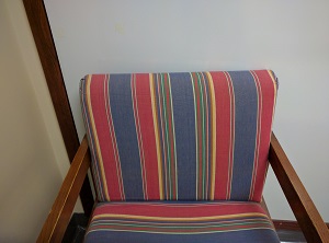
Let us take a look at this idea visually. Consider this image of a chair:
A visual representation of how this image is stored as a NumPy array is:
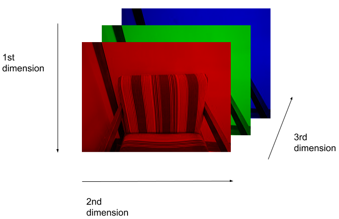
So, when we are working with skimage images, we specify the y coordinate first, then the x coordinate. And, the colors are stored as RGB values – red in layer 0, green in layer 1, blue in layer 2.
Coordinate and color channel order
CAUTION: it is vital to remember the order of the coordinates and color channels when dealing with images as NumPy arrays. If we are manipulating or accessing an image array directly, we specifiy the y coordinate first, then the x. Further, the first channel stored is the red channel, followed by the green, and then the blue.
Reading, displaying, and saving images
Skimage provides easy-to-use functions for reading, displaying, and saving images. All of the popular image formats, such as BMP, PNG, JPEG, and TIFF are supported, along with several more esoteric formats. See the skimage documentation for more information.
Let us examine a simple Python program to load, display, and save an image to a different format. Here are the first few lines:
"""
 * Python program to open, display, and save an image.
 *
"""
import skimage.io

# read image
image = skimage.io.imread(fname="chair.jpg")
First, we import the io module of skimage (skimage.io) so
we can read and write images. Then, we use the skimage.io.imread() function to read
a JPEG image entitled chair.jpg. Skimage reads the image, converts it from
JPEG into a NumPy array, and returns the array; we save the array in a variable
named image.
Next, we will do something with the image:
import skimage.viewer

# display image
viewer = skimage.viewer.ImageViewer(image)
viewer.show()
Once we have the image in the program, we next import the viewer module of skimage
(skimage.viewer) and display it using skimage.viewer.ImageViewer(), which
returns a ImageViewer object we store in the viewer variable.
We then call viewer.show() in order to display the image.
Next, we will save the image in another format:
# save a new version in .tif format
skimage.io.imsave(fname="chair.tif", arr=image)
The final statement in the program, skimage.io.imsave(fname="chair.tif", arr=image),
writes the image to a file named chair.tif. The imsave() function automatically
determines the type of the file, based on the file extension we provide. In
this case, the .tif extension causes the image to be saved as a TIFF.
Extensions do not always dictate file type
The skimage
imsave()function automatically uses the file type we specify in the file name parameter’s extension. Note that this is not always the case. For example, if we are editing a document in Microsoft Word, and we save the document aspaper.pdfinstead ofpaper.docx, the file is not saved as a PDF document.
Named versus positional arguments
When we call functions in Python, there are two ways we can specify the necessary arguments. We can specify the arguments positionally, i.e., in the order the parameters appear in the function definition, or we can use named arguments.
For example, the
skimage.io.imread()function definition specifies two parameters, the file name to read and an optional flag value. So, we could load in the chair image in the sample code above using positional parameters like this:
image = skimage.io.imread('chair.jpg')Since the function expects the first argument to be the file name, there is no confusion about what
'char.jpg'means.The style we will use in this workshop is to name each parameters, like this:
image = skimage.io.imsave(fname='chair.jpg')This style will make it easier for you to learn how to use the variety of functions we will cover in this workshop.
Resizing an image (20 min)
Using your mobile phone, tablet, web cam, or digital camera, take an image. Copy the image to the Desktop/workshops/image-processing/03-skimage-images directory. Write a Python program to read your image into a variable named
image. Then, resize the image by a factor of 50 percent, using this line of code:new_shape = (image.shape[0] // 2, image.shape[1] // 2, image.shape[2]) small = skimage.transform.resize(image=image, output_shape=new_shape)As it is used here, the parameters to the
skimage.transform.resize()function are the image to transform,image, the dimensions we want the new image to have.Finally, write the resized image out to a new file named resized.jpg. Once you have executed your program, examine the image properties of the output image and verify it has been resized properly.
Solution
Here is what your Python program might look like.
"""
 * Python program to read an image, resize it, and save it
 * under a different name.
"""
import skimage.io
import skimage.transform

# read in image
image = skimage.io.imread(fname="chicago.jpg")

# resize the image
new_shape = (image.shape[0] // 2, image.shape[1] // 2, image.shape[2])
small = skimage.transform.resize(image=image, output_shape=new_shape)

# write out image
skimage.io.imsave(fname="resized.jpg", arr=small)
From the command line, we would execute the program like this:
python Resize.pyThe program resizes the chicago.jpg image by 50% in both dimensions, and saves the result in the resized.jpg file.
Manipulating pixels
If we desire or need to, we can individually manipulate the colors of pixels by changing the numbers stored in the image’s NumPy array.
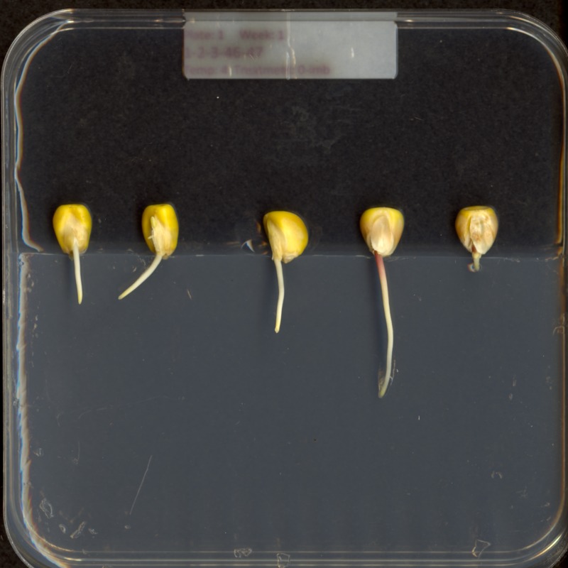
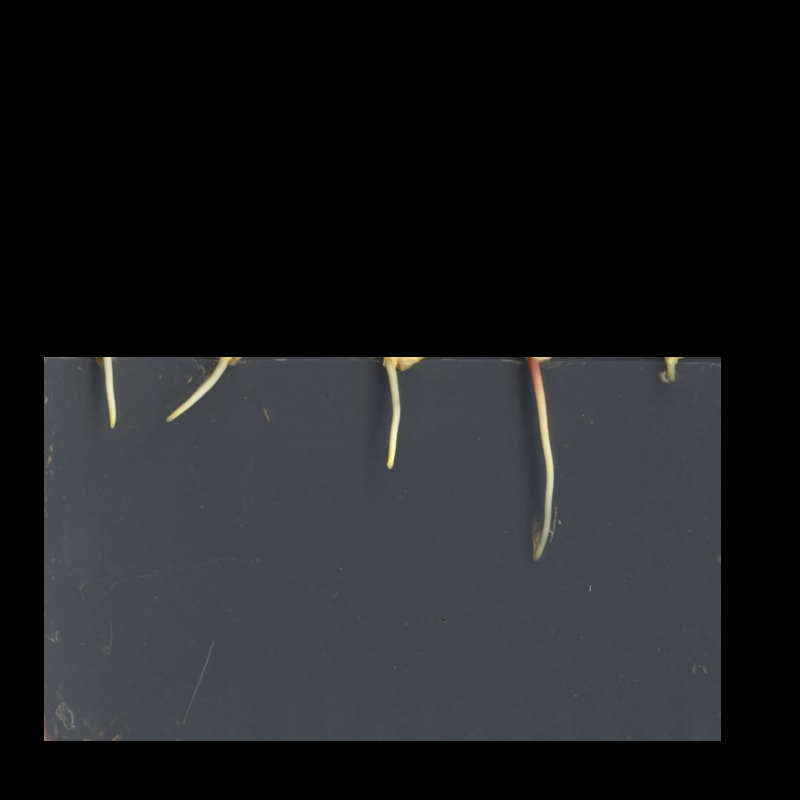
For example, suppose we are interested in this maize root cluster image. We want to be able to focus our program’s attention on the roots themselves, while ignoring the black background.
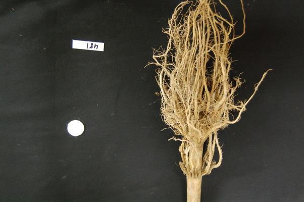
Since the image is stored as an array of numbers, we can simply look through the array for pixel color values that are less than some threshold value. This process is called thresholding, and we will see more powerful methods to perform the thresholding task in the Thresholding episode. Here, though, we will look at a simple and elegant NumPy method for thresholding. Let us develop a program that keeps only the pixel color values in an image that have value greater than or equal to 128. This will keep the pixels that are brighter than half of “full brightness;” i.e., pixels that do not belong to the black background. We will start by reading the image and displaying it.
"""
* Python script to ignore low intensity pixels in an image.
*
* usage: python HighIntensity.py <filename>
"""
import sys
import skimage.io
import skimage.viewer

# read input image, based on filename parameter
image = skimage.io.imread(fname=sys.argv[1])

# display original image
viewer = skimage.viewer.ImageViewer(image)
viewer.show()
Our program imports sys in addition to skimage, so that we can use
command-line arguments when we execute the program. In particular, in this
program we use a command-line argument to specify the filename of the image to
process. If the name of the file we are interested in is roots.jpg, and
the name of the program is HighIntensity.py, then we run our Python
program form the command line like this:
python HighIntensity.py roots.jpg
The place where this happens in the code is the
skimage.io.imread(fname=sys.argv[1])
function call. When we invoke our program with command line arguments,
they are passed in to the program as a list; sys.argv[1] is the first one
we are interested in; it contains the image filename we want to process.
(sys.argv[0] is simply the name of our program, HighIntensity.py in
this case).
Benefits of command-line arguments
Passing parameters such as filenames into our programs as parameters makes our code more flexible. We can now run HighIntensity.py on any image we wish, without having to go in and edit the code.
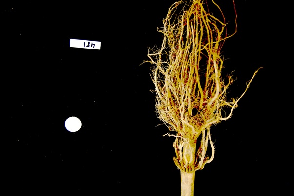
Now we can threshold the image and display the result.
# keep only high-intensity pixels
image[image < 128] = 0

# display modified image
viewer = skimage.viewer.ImageViewer(image)
viewer.show()
The NumPy command to ignore all low-intensity pixels is img[img < 128] = 0.
Every pixel color value in the whole 3-dimensional array with a value less
that 128 is set to zero. In this case, the result is an image in which the
extraneous background detail has been removed.
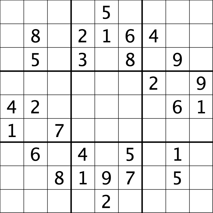
Keeping only low intensity pixels (20 min)
In the previous example, we showed how we could use Python and skimage to turn on only the high intensity pixels from an image, while turning all the low intensity pixels off. Now, you can practice doing the opposite – keeping all the low intensity pixels while changing the high intensity ones. Consider this image of a Su-Do-Ku puzzle, named sudoku.png:
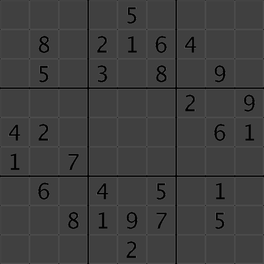
Navigate to the Desktop/workshops/image-processing/03-skimage-images directory, and copy the HighIntensity.py program to another file named LowIntensity.py. Then, edit the LowIntensity.py program so that it turns all of the white pixels in the image to a light gray color, say with all three color channel values for each formerly white pixel set to 64. Your results should look like this:
Solution
After modification, your program should look like this:
"""
* Python script to modify high intensity pixels in an image.
*
* usage: python LowIntensity.py <filename>
"""
import sys
import skimage.io
import skimage.viewer

# read input image, based on filename parameter
img = skimage.io.imread(fname=sys.argv[1])

# display original image
viewer = skimage.viewer.ImageViewer(img)
viewer.view()

# change high intensity pixels to gray
img[img > 200] = 64

# display modified image
viewer = skimage.viewer.ImageViewer(img)
viewer.view()
Converting color images to grayscale
It is often easier to work with grayscale images, which have a single channel,
instead of color images, which have three channels.
Skimage offers the function skimage.color.rgb2gray() to achieve this.
This function adds up the three color channels in a way that matches
human color perception, see the skimage documentation for details.
It returns a grayscale image with floating point values in the range from 0 to 1.
We can use the function skimage.util.img_as_ubyte() in order to convert it back to the
original data type and the data range back 0 to 255.
Note that it is often better to use image values represented by floating point values,
because using floating point numbers is numerically more stable.
"""
* Python script to load a color image as grayscale.
*
* usage: python LoadGray.py <filename>
"""
import sys
import skimage.io
import skimage.viewer
import skimage.color

# read input image, based on filename parameter
image = skimage.io.imread(fname=sys.argv[1])

# display original image
viewer = skimage.viewer.ImageViewer(image)
viewer.show()

# convert to grayscale and display
gray_image = skimage.color.rgb2gray(image)
viewer = skimage.viewer.ImageViewer(gray_image)
viewer.show()
We can also load color images as grayscale directly by passing the argument as_gray=True to
skimage.io.imread().
"""
* Python script to load a color image as grayscale.
*
* usage: python LoadGray.py <filename>
"""
import sys
import skimage.io
import skimage.viewer
import skimage.color

# read input image, based on filename parameter
image = skimage.io.imread(fname=sys.argv[1], as_gray=True)

# display grayscale image
viewer = skimage.viewer.ImageViewer(image)
viewer.show()
Access via slicing
Since skimage images are stored as NumPy arrays, we can use array slicing to select rectangular areas of an image. Then, we could save the selection as a new image, change the pixels in the image, and so on. It is important to remember that coordinates are specified in (y, x) order and that color values are specified in (r, g, b) order when doing these manipulations.
Consider this image of a whiteboard, and suppose that we want to create a sub-image with just the portion that says “odd + even = odd,” along with the red box that is drawn around the words.
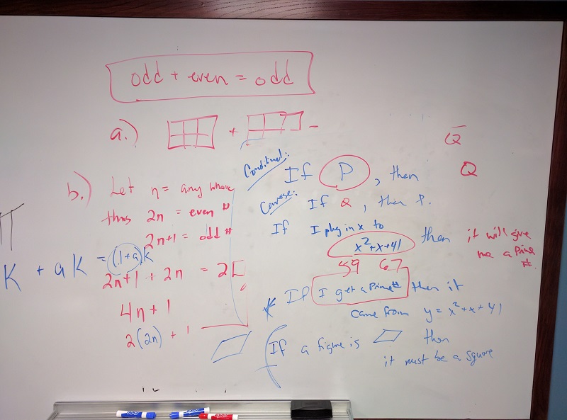
We can use a tool such as ImageJ to determine the coordinates of the corners of the area we wish to extract. If we do that, we might settle on a rectangular area with an upper-left coordinate of (135, 60) and a lower-right coordinate of (480, 150), as shown in this version of the whiteboard picture:
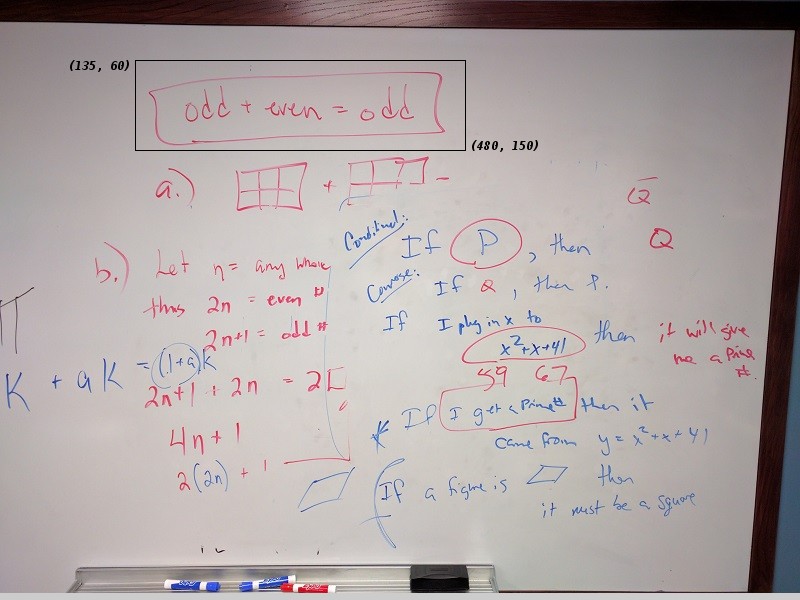
Note that the coordinates in the preceding image are specified in (x, y)
order. Now if our entire whiteboard image is stored as an skimage image named
image, we can create a new image of the selected region with a statement like
this:
clip = image[60:151, 135:481, :]
Our array slicing specifies the range of y-coordinates first, 60:151, and
then the range of x-coordinates, 135:481. Note we go one beyond the maximum
value in each dimension, so that the entire desired area is selected.
The third part of the slice, :, indicates that we want all three color
channels in our new image.
A program to create the subimage would start by loading the image:
"""
 * Python script demonstrating image modification and creation via
 * NumPy array slicing.
"""
import skimage.io
import skimage.viewer

# load and display original image
image = skimage.io.imread(fname="board.jpg")
viewer = skimage.viewer.ImageViewer(image)
viewer.show()
Then we use array slicing to create a new image with our selected area and then display the new image.
# extract, display, and save sub-image
clip = image[60:151, 135:481, :]
viewer = skimage.viewer.ImageViewer(clip)
viewer.show()
skimage.io.imsave(fname="clip.tif", arr=clip)
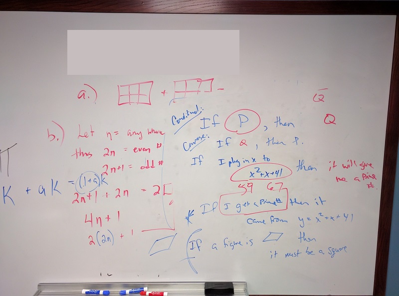
We can also change the values in an image, as shown next.
# replace clipped area with sampled color
color = image[330, 90]
image[60:151, 135:481] = color
viewer = skimage.viewer.ImageViewer(image)
viewer.show()
First, we sample the color at a particular location of the
image, saving it in a NumPy array named color, a 1 × 1 × 3 array with the blue,
green, and red color values for the pixel located at (x = 90, y = 330). Then,
with the img[60:151, 135:481] = color command, we modify the image in the
specified area. In this case, the command “erases” that area of the whiteboard,
replacing the words with a white color, as shown in the final image produced by
the program:
Practicing with slices (10 min)
Navigate to the Desktop/workshops/image-processing/03-skimage-images directory, and edit the RootSlice.py program. It contains a skeleton program that loads and displays the maize root image shown above. Modify the program to create, display, and save a sub-image containing only the plant and its roots. Use ImageJ to determine the bounds of the area you will extract using slicing.
Solution
Here is the completed Python program to select only the plant and roots in the image.
"""
 * Python script to extract a sub-image containing only the plant and
 * roots in an existing image.
"""
import skimage.io
import skimage.viewer

# load and display original image
image = skimage.io.imread(fname="roots.jpg")
viewer = skimage.viewer.ImageViewer(image)
viewer.show()

# extract, display, and save sub-image
# WRITE YOUR CODE TO SELECT THE SUBIMAGE NAME clip HERE:
clip = image[0:1999, 1410:2765, :]
viewer = skimage.viewer.ImageViewer(clip)
viewer.show()


# WRITE YOUR CODE TO SAVE clip HERE
skimage.io.imsave(fname="clip.jpg", arr=clip)
Metadata, continued (10 min)
Let us return to the concept of image metadata, introduced briefly in the Image Basics episode. Specifically, what happens to the metadata of an image when it is read into, and written from, a Python program using skimage?
To answer this question, write a very short (three lines) Python script to read in a file and save it under a different name. Navigate to the Desktop/workshops/image-processing/03-skimage-images directory, and write your script there. You can use the flowers-before.jpg as input, and save the output as flowers-after.jpg. Then, examine the metadata from both images using commands like identify -verbose flowers-after.jpg. Is the metadata the same? If not, what are some key differences?
Solution
Here is a short Python script to open the image and save it in a different filename:
import skimage.io

img = skimage.io.imread(fname="flowers-before.jpg")
skimage.io.imsave(fname="flowers-after.jpg", arr=img)
The newly-saved file is missing most of the original metadata. Comparing this to the original, as shown in the Image Basics episode, it is easy to see that virtually all of the useful metadata has been lost!
The moral of this challenge is to remember that image metadata will not be preserved in images that your programs write via the
skimage.io.imsave()function. If metadata is important to you, take precautions to always preserve the original files.
Slicing and the colorimetric challenge (10 min)
In the introductory episode, we were introduced to a colorimetric challenge, namely, graphing the color values of a solution in a titration, to see when the color change takes place. Let’s start thinking about how to solve that problem.
One part of our ultimate solution will be sampling the color channel values from an image of the solution. To make our graph more reliable, we will want to calculate a mean channel value over several pixels, rather than simply focusing on one pixel from the image.
Navigate to the Desktop/workshops/image-processing/10-challenges/colorimetrics directory, and open the titration.tiff image in ImageJ.
Find the (x, y) coordinates of an area of the image you think would be good to sample in order to find the average channel values. Then, write a small Python program that computes the mean channel values for a 10 × 10 pixel kernel centered around the coordinates you chose. Print the results to the screen, in a format like this:
Avg. red value: 193.7778
Avg. green value: 189.1481
Avg. blue value: 178.6049
Key Points
skimage images are stored as three-dimensional NumPy arrays.
In skimage images, the red channel is specified first, then the green, then the blue, i.e. RGB.
Images are read from disk with the
skimage.io.imread()function.We create a window that automatically scales the displayed image with
skimage.viewer.ImageViewer()and callingview()on the viewer object.Color images can be transformed to grayscale using
skimage.color.rgb2gray()or be read as grayscale directly by passing the argumentas_gray=Truetoskimage.io.imread().We can resize images with the
skimage.transform.resize()function.NumPy array commands, like
img[img < 128] = 0, and be used to manipulate the pixels of an image.Command-line arguments are accessed via the
sys.argvlist;sys.argv[1]is the first parameter passed to the program,sys.argv[2]is the second, and so on.Array slicing can be used to extract sub-images or modify areas of images, e.g.,
clip = img[60:150, 135:480, :].Metadata is not retained when images are loaded as skimage images.
Drawing and Bitwise Operations
Overview
Teaching: 20 min
Exercises: 60 minQuestions
How can we draw on skimage images and use bitwise operations and masks to select certain parts of an image?
Objectives
Create a blank, black skimage image.
Draw rectangles and other shapes on skimage images.
Explain how a white shape on a black background can be used as a mask to select specific parts of an image.
Use bitwise operations to apply a mask to an image.
The next series of episodes covers a basic toolkit of skimage operators. With these tools, we will be able to create programs to perform simple analyses of images based on changes in color or shape.
Drawing on images
Often we wish to select only a portion of an image to analyze, and ignore the rest. Creating a rectangular sub-image with slicing, as we did in the skimage Images lesson is one option for simple cases. Another option is to create another special image, of the same size as the original, with white pixels indicating the region to save and black pixels everywhere else. Such an image is called a mask. In preparing a mask, we sometimes need to be able to draw a shape – a circle or a rectangle, say – on a black image. skimage provides tools to do that.
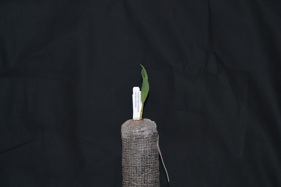
Consider this image of maize seedlings:
Now, suppose we want to analyze only the area of the image containing the roots themselves; we do not care to look at the kernels, or anything else about the plants. Further, we wish to exclude the frame of the container holding the seedlings as well. Exploration with ImageJ could tell us that the upper-left coordinate of the sub-area we are interested in is (44, 357), while the lower-right coordinate is (720, 740). These coordinates are shown in (x, y) order.
A Python program to create a mask to select only that area of the image would start with a now-familiar section of code to open and display the original image. (Note that the display portion is used here for pedagogical purposes; it would probably not be used in production code.)
"""
 * Python program to use skimage drawing tools to create a mask.
 *
"""
import skimage
from skimage.viewer import ImageViewer
import numpy as np

# Load and display the original image
image = skimage.io.imread("maize-roots.tif")
viewer = ImageViewer(image)
viewer.show()
As before, we first import skimage. We also import the NumPy library, and give
it an alias of np. NumPy is necessary when we create the initial mask image,
and the alias saves us a little typing. Then, we load and display the initial
image in the same way we have done before.
NumPy allows indexing of images/arrays with “boolean” arrays of the same size.
Indexing with a boolean array is also called mask indexing. The “pixels” in such
a mask array can only take two values: True or False. When indexing an image
with such a mask, only pixel values at positions where the mask is True are
accessed. But first, we need to generate a mask array of the same size as the
image. Luckily, the NumPy library provides a function to create just such an
array. The next section of code shows how.
# Create the basic mask
mask = np.ones(shape=image.shape[0:2], dtype="bool")
We create the mask image with the
mask = np.ones(shape=image.shape[0:2], dtype="bool")
function call. The first argument to the ones() function is the shape of
the original image, so that our mask will be exactly the same size as the
original. Notice, that we have only used the first two indices of our shape. We
omitted the channel dimension. Indexing with such a mask will change all channel
values simultaneously. The second argument, dtype = "bool", indicates that the
elements in the array should be booleans – i.e., values are either True or
False. Thus, even though we use np.ones() to create the mask, its pixel values
are in fact not 1 but True. You could check this,
e.g., by print(mask[0, 0]).
Next, we draw a filled, rectangle on the mask:
# Draw filled rectangle on the mask image
rr, cc = skimage.draw.rectangle(start=(357, 44), end=(740, 720))
mask[rr, cc] = False
The parameters of the rectangle() function (357, 44) and (740, 720), are the coordinates of the
upper-left (start) and lower-right (end) corners of a rectangle in (y, x) order.
The function returns the rectangle as row (rr) and column (cc) coordinate arrays.
Check the documentation!
When using an skimage function for the first time – or the fifth time – it is wise to check how the function is used, via the online skimage documentation or via other usage examples on programming-related sites such as Stack Overflow. Basic information about skimage functions can be found interactively in Python, via commands like
help(skimage)orhelp(skimage.draw.rectangle). Take notes in your lab notebook. And, it is always wise to run some test code to verify that the functions your program uses are behaving in the manner you intend.
Variable naming conventions!
You may have wondered why we called the return values of the rectangle function
rrandcc?! You may have guessed thatris short forrowandcis short forcolumn. However, the rectangle function returns mutiple rows and columns; thus we used a convention of doubling the letterrtorr(andctocc) to indicate that those are multiple values. In fact it may have even been clearer to name those variablesrowsandcolumns; however this would have been also much longer. Whatever you decide to do, try to stick to some already existing conventions, such that it is easier for other people to understand your code.
The final section of the program displays the mask we just created:
# Display constructed mask
viewer = ImageViewer(mask)
viewer.show()
Here is what our constructed mask looks like:
Other drawing operations (10 min)
There are other functions for drawing on images, in addition to the
skimage.draw.rectangle()function. We can draw circles, lines, text, and other shapes as well. These drawing functions may be useful later on, to help annotate images that our programs produce. Practice some of these functions here. Navigate to the Desktop/workshops/image-processing/04-drawing-bitwise directory, and edit the DrawPractice.py program. The program creates a black, 800x600 pixel image. Your task is to draw some other colored shapes and lines on the image, perhaps something like this:
Circles can be drawn with the
skimage.draw.circle()function, which takes three parameters: x, y point of the center of the circle, and the radius of the filled circle. There is an optionalshapeparameter that can be supplied to this function. It will limit the output coordinates for cases where the circle dimensions exceed the ones of the image.Lines can be drawn with the
skimage.draw.line()function, which takes four parameters: the image to draw on, the (x, y) coordinate of one end of the segment, the (x, y) coordinate of the other end of the segment, and the color for the line.Other drawing functions supported by skimage can be found in the skimage reference pages.
Solution
Here is an overly-complicated version of the drawing program, to draw shapes that are randomly placed on the image.
"""
 * Program to practice with skimage drawing methods.
"""
import random
import numpy as np
import skimage
from skimage.viewer import ImageViewer

# create the black canvas
image = np.zeros(shape=(600, 800, 3), dtype="uint8")

# WRITE YOUR CODE TO DRAW ON THE IMAGE HERE
for i in range(15):
    x = random.random()
    if x < 0.33:
        rr, cc = skimage.draw.circle(
            random.randrange(600),
            random.randrange(800),
            radius=50,
            shape=image.shape[0:2],
        )
        color = (0, 0, 255)
    elif x < 0.66:
        rr, cc = skimage.draw.line(
            random.randrange(600),
            random.randrange(800),
            random.randrange(600),
            random.randrange(800),
        )
        color = (0, 255, 0)
    else:
        rr, cc = skimage.draw.rectangle(
            start=(random.randrange(600), random.randrange(800)),
            extent=(50, 50),
            shape=image.shape[0:2],
        )
        color = (255, 0, 0)

    image[rr, cc] = color

# display the results
viewer = ImageViewer(image)
viewer.show()
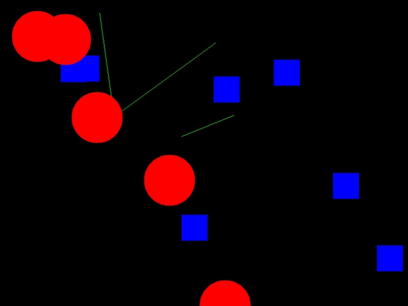
Image modification
All that remains is the task of modifying the image using our mask in such a
way that the areas with True pixels in the mask are not shown in the image
any more.
How does a mask work?
Now, consider the mask image we created above. The values of the mask that corresponds to the portion of the image we are interested in are all
False, while the values of the mask that corresponds to the portion of the image we want to remove are allTrue.How do we change the original image using the mask?
Solution
When indexing the image using the mask, we access only those pixels at positions where the mask is
True. So, when indexing with the mask, one can set those values to 0, and effectively remove them from the image.
Now we can write a Python program to use a mask to retain only the portions of our maize roots image that actually contains the seedling roots. We load the original image and create the mask in the same way as before:
"""
 * Python program to apply a mask to an image.
 *
"""
import numpy as np
import skimage
from skimage.viewer import ImageViewer

# Load the original image
image = skimage.io.imread("maize-roots.tif")

# Create the basic mask
mask = np.ones(shape=image.shape[0:2], dtype="bool")

# Draw a filled rectangle on the mask image
rr, cc = skimage.draw.rectangle(start=(357, 44), end=(740, 720))
mask[rr, cc] = False
Then, we use numpy indexing to remove the portions of the image, where the mask
is True:
# Apply the mask and display the result
image[mask] = 0
Then, we display the masked image.
viewer = ImageViewer(image)
viewer.show()
The resulting masked image should look like this:
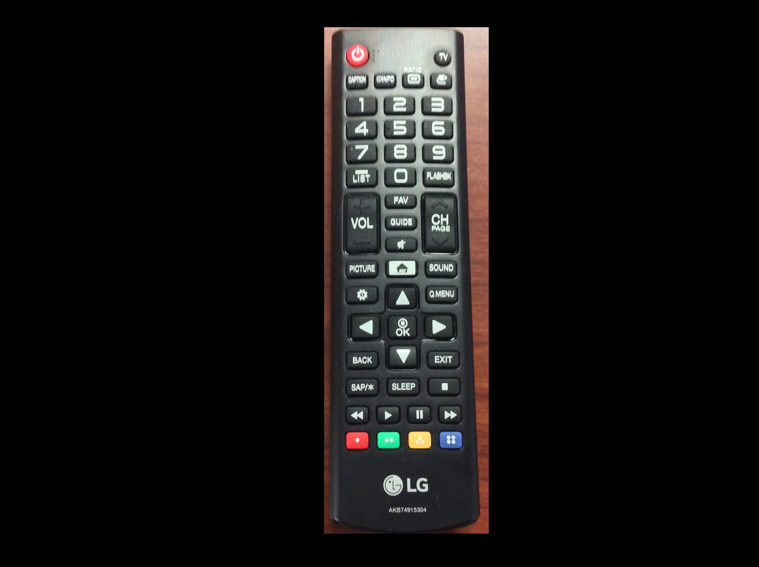
Masking an image of your own (optional)
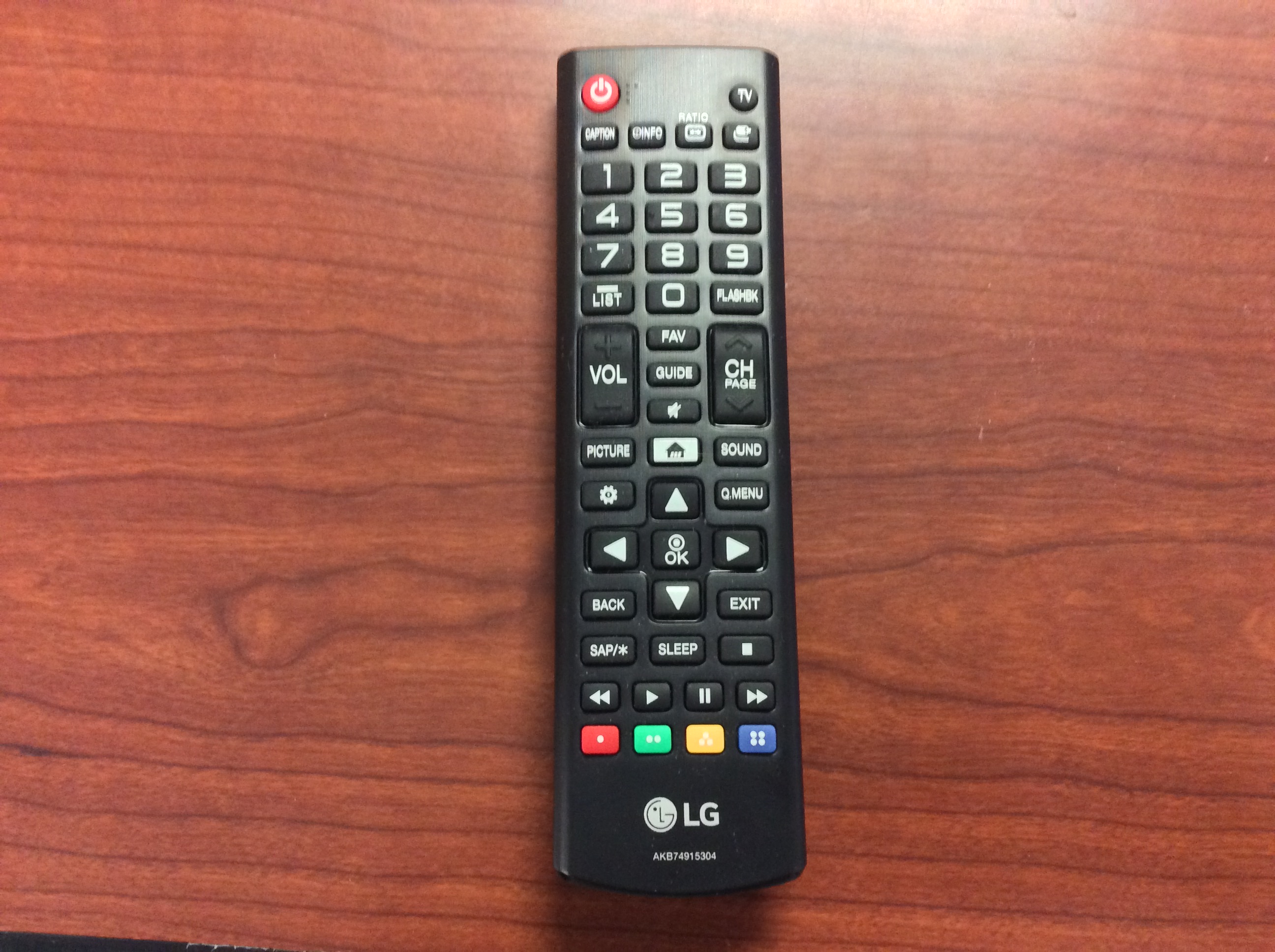
Now, it is your turn to practice. Using your mobile phone, tablet, webcam, or digital camera, take an image of an object with a simple overall geometric shape (think rectangular or circular). Copy that image to the Desktop/workshops/image-processing/04-drawing-bitwise directory. Copy the MaskAnd.py program to another file named MyMask.py. Then, edit the MyMask.py program to use a mask to select only the primary object in your image. For example, here is an image of a remote control:
And, here is the end result of a program masking out everything but the remote.
Solution
Here is a Python program to produce the cropped remote control image shown above. Of course, your program should be tailored to your image.
"""
 * Python program to apply a mask to an image.
 *
"""
import numpy as np
import skimage
from skimage.viewer import ImageViewer

# Load the original image
image = skimage.io.imread("./fig/03-remote-control.jpg")

# Create the basic mask
mask = np.ones(shape=image.shape[0:2], dtype="bool")

# Draw a filled rectangle on the mask image
rr, cc = skimage.draw.rectangle(start=(93, 1107), end=(1821, 1668))
mask[rr, cc] = False

# Apply the mask and display the result
image[mask] = 0
viewer = ImageViewer(image)
viewer.show()
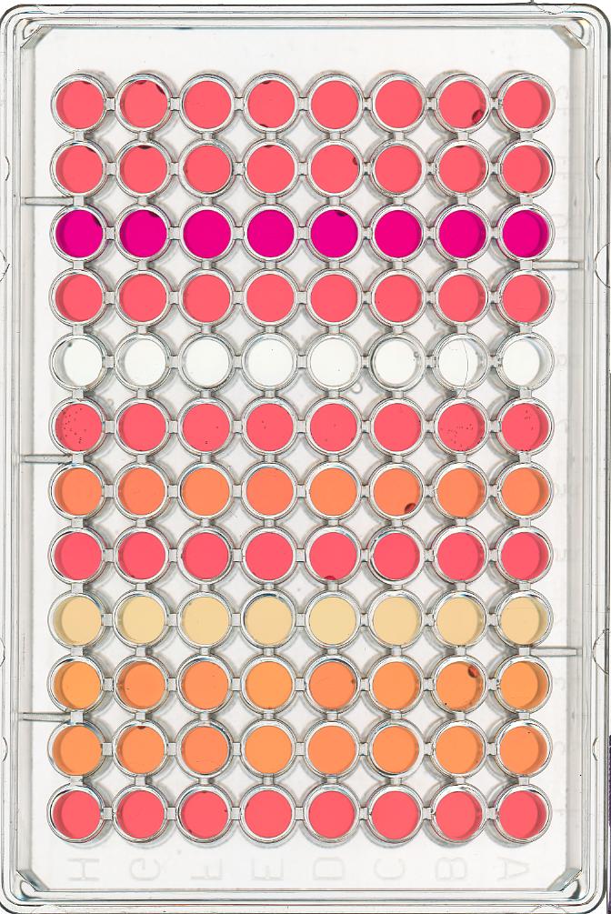
Masking a 96-well plate image (50 min)
Consider this image of a 96-well plate that has been scanned on a flatbed scanner.
Suppose that we are interested in the colors of the solutions in each of the wells. We do not care about the color of the rest of the image, i.e., the plastic that makes up the well plate itself.
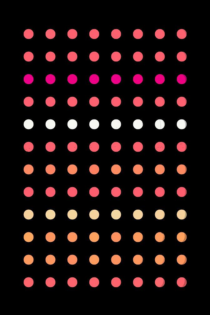
Navigate to the Desktop/workshops/image-processing/04-drawing-bitwise directory; there you will find the well plate image shown above, in the file named wellplate.tif. In this directory you will also find a text file containing the (x, y) coordinates of the center of each of the 96 wells on the plate, with one pair per line; this file is named centers.txt. You may assume that each of the wells in the image has a radius of 16 pixels. Write a Python program that reads in the well plate image, and the centers text file, to produce a mask that will mask out everything we are not interested in studying from the image. Your program should produce output that looks like this:
Solution
This program reads in the image file based on the first command-line parameter, and writes the resulting masked image to the file named in the second command line parameter.
"""
 * Python program to mask out everything but the wells
 * in a standardized scanned 96-well plate image.
"""
import numpy as np
import skimage
from skimage.viewer import ImageViewer
import sys

# read in original image
image = skimage.io.imread(sys.argv[1])

# create the mask image
mask = np.ones(shape=image.shape[0:2], dtype="bool")

# open and iterate through the centers file...
with open("centers.txt", "r") as center_file:
    for line in center_file:
        # ... getting the coordinates of each well...
        tokens = line.split()
        x = int(tokens[0])
        y = int(tokens[1])

        # ... and drawing a white circle on the mask
        rr, cc = skimage.draw.circle(y, x, radius=16, shape=image.shape[0:2])
        mask[rr, cc] = False

# apply the mask
image[mask] = 0

# write the masked image to the specified output file
skimage.io.imsave(fname=sys.argv[2], arr=image)
Masking a 96-well plate image, take two (optional)
If you spent some time looking at the contents of the centers.txt file from the previous challenge, you may have noticed that the centers of each well in the image are very regular. Assuming that the images are scanned in such a way that the wells are always in the same place, and that the image is perfectly oriented (i.e., it does not slant one way or another), we could produce our well plate mask without having to read in the coordinates of the centers of each well. Assume that the center of the upper left well in the image is at location x = 91 and y = 108, and that there are 70 pixels between each center in the x dimension and 72 pixels between each center in the y dimension. Each well still has a radius of 16 pixels. Write a Python program that produces the same output image as in the previous challenge, but without having to read in the centers.txt file. Hint: use nested for loops.
Solution
Here is a Python program that is able to create the masked image without having to read in the centers.txt file.
"""
 * Python program to mask out everything but the wells
 * in a standardized scanned 96-well plate image, without
 * using a file with well center location.
"""
import numpy as np
import skimage
from skimage.viewer import ImageViewer
import sys

# read in original image
image = skimage.io.imread(sys.argv[1])

# create the mask image
mask = np.ones(shape=image.shape[0:2], dtype="bool")

# upper left well coordinates
x0 = 91
y0 = 108

# spaces between wells
deltaX = 70
deltaY = 72

x = x0
y = y0

# iterate each row and column
for row in range(12):
    # reset x to leftmost well in the row
    x = x0
    for col in range(8):

        # ... and drawing a white circle on the mask
        rr, cc = skimage.draw.circle(y, x, radius=16, shape=image.shape[0:2])
        mask[rr, cc] = False
        x += deltaX
    # after one complete row, move to next row
    y += deltaY

# apply the mask
image[mask] = 0

# write the masked image to the specified output file
skimage.io.imsave(fname=sys.argv[2], arr=image)
Key Points
We can use the NumPy
zeros()function to create a blank, black image.We can draw on skimage images with functions such as
skimage.draw.rectangle(),skimage.draw.circle(),skimage.draw.line(), and more.The drawing functions return indices to pixels that can be set directly.
Creating Histograms
Overview
Teaching: 25 min
Exercises: 60 minQuestions
How can we create grayscale and color histograms to understand the distribution of color values in an image?
Objectives
Explain what a histogram is.
Load an image in grayscale format.
Create and display grayscale and color histograms for entire images.
Create and display grayscale and color histograms for certain areas of images, via masks.
In this episode, we will learn how to use skimage functions to create and display histograms for images.
Introduction to Histograms
As it pertains to images, a histogram is a graphical representation showing how frequently various color values occur in the image. We saw in the Image Basics episode that we could use a histogram to visualize the differences in uncompressed and compressed image formats. If your project involves detecting color changes between images, histograms will prove to be very useful, and histograms are also quite handy as a preparatory step before performing Thresholding or Edge Detection.
Grayscale Histograms
We will start with grayscale images and histograms first, and then move on to color images. Here is a Python script to load an image in grayscale instead of full color, and then create and display the corresponding histogram. The first few lines are:
"""
 * Generate a grayscale histogram for an image.
 *
 * Usage: python GrayscaleHistogram.py <fiilename>
"""
import sys
import numpy as np
import skimage.color
import skimage.io
import skimage.viewer
from matplotlib import pyplot as plt

# read image, based on command line filename argument;
# read the image as grayscale from the outset
image = skimage.io.imread(fname=sys.argv[1], as_gray=True)

# display the image
viewer = skimage.viewer.ImageViewer(image)
viewer.show()
In the program, we have a new import from matplotlib, to gain access to the
tools we will use to draw the histogram. The statement
from matplotlib import pyplot as plt
loads up the pyplot library, and gives it a shorter name, plt.
Next, we use the skimage.io.imread() function to load our image. We use the first
command line parameter as the filename of the image, as we did in the
Skimage Images lesson. The second parameter
to skimage.io.imread() instructs the function to transform the image into
grayscale with a value range from 0 to 1 while loading the image.
We will keep working with images in the value range 0 to 1 in this lesson.
Remember that we can transform an image back to the range 0 to 255 with
the function skimage.util.img_as_ubyte.
Skimage does not provide a special function to compute histograms, but we can use
the function np.histogram instead:
# create the histogram
histogram, bin_edges = np.histogram(image, bins=256, range=(0, 1))
The parameter bins determines the histogram size, or the number of “bins” to use for
the histogram. We pass in 256 because we want to see the pixel count for
each of the 256 possible values in the grayscale image.
The parameter range is the range of values each of the pixels in the image can
have. Here, we pass 0 and 1, which is the value range of our input image after transforming it
to grayscale.
The first output of the np.histogram function is a one-dimensional NumPy array,
with 256 rows and one column, representing the number of pixels with the color
value corresponding to the index. I.e., the first number in the array is the
number of pixels found with color value 0, and the final
number in the array is the number of pixels found with color value 255.
The second output of np.histogram is an array with the bin edges and one column and 257 rows (one more than the histogram itself).
There are no gaps between the bins, which means that the end of the first bin, is the start of the second and so on.
For the last bin, the array also has to contain the stop, so it has one more element, than the histogram.
Next, we turn our attention to displaying the histogram, by taking advantage
of the plotting facilities of the matplotlib library.
# configure and draw the histogram figure
plt.figure()
plt.title("Grayscale Histogram")
plt.xlabel("grayscale value")
plt.ylabel("pixels")
plt.xlim([0.0, 1.0])  # <- named arguments do not work here

plt.plot(bin_edges[0:-1], histogram)  # <- or here
plt.show()
We create the plot with
plt.figure(), then label the figure and the coordinate axes with
plt.title(), plt.xlabel(), and plt.ylabel() functions. The last step in
the preparation of the figure is to set the limits on the values on the
x-axis with the plt.xlim([0.0, 1.0]) function call.
Variable-length argument lists
Note that we cannot used named parameters for the
plt.xlim()orplt.plot()functions. This is because these functions are defined to take an arbitrary number of unnamed arguments. The designers wrote the functions this way because they are very versatile, and creating named parameters for all of the possible ways to use them would be complicated.
Finally, we create the histogram plot itself with plt.plot(bin_edges[0:-1], histogram).
We use the left bin edges as x-positions for the histogram values by indexing the bin_edges array to ignore the last value (the right edge of the last bin).
Then we make it appear with plt.show(). When we run the program on this image of a plant seedling,
Histograms in matplotlib
Matplotlib provides a dedicated function to compute and display histograms:
plt.hist(). We will not use it in this lesson in order to understand how to calculate histograms in more detail. In practice, it is a good idea to use this function, because it visualizes histograms more appropriately thanplt.plot(). Here, you could use it by callingplt.hist(image.flatten(), bins=256, range=(0, 1))instead ofnp.histogram()andplt.plot()(*.flatten()is a numpy function that converts our two-dimensional image into a one-dimensional array).
the program produces this histogram:
Using a mask for a histogram (25 min)
Looking at the histogram above, you will notice that there is a large number of very dark pixels, as indicated in the chart by the spike around the grayscale value 0.12. That is not so surprising, since the original image is mostly black background. What if we want to focus more closely on the leaf of the seedling? That is where a mask enters the picture!
Navigate to the Desktop/workshops/image-processing/05-creating-histograms directory, and edit the GrayscaleMaskHistogram.py program. The skeleton program is a copy of the mask program above, with comments showing where to make changes.
First, use a tool like ImageJ to determine the (x, y) coordinates of a bounding box around the leaf of the seedling. Then, using techniques from the Drawing and Bitwise Operations episode, create a mask with a white rectangle covering that bounding box.
After you have created the mask, apply it to the input image before passing it to the
np.histogramfunction. Then, run the GrayscaleMaskHistogram.py program and observe the resulting histogram.Solution
"""
 * Generate a grayscale histogram for an image.
 *
 * Usage: python GrayscaleMaskHistogram.py <filename>
"""
import sys
import numpy as np
import skimage.draw
import skimage.io
import skimage.viewer
from matplotlib import pyplot as plt

# read image, based on command line filename argument;
# read the image as grayscale from the outset
img = skimage.io.imread(fname=sys.argv[1], as_gray=True)

# display the image
viewer = skimage.viewer.ImageViewer(img)
viewer.show()

# create mask here, using np.zeros() and skimage.draw.rectangle()
mask = np.zeros(shape=img.shape, dtype="bool")
rr, cc = skimage.draw.rectangle(start=(199, 410), end=(384, 485))
mask[rr, cc] = True

# mask the image and create the new histogram
histogram, bin_edges = np.histogram(img[mask], bins=256, range=(0.0, 1.0))

# configure and draw the histogram figure
plt.figure()

plt.title("Grayscale Histogram")
plt.xlabel("grayscale value")
plt.ylabel("pixel count")
plt.xlim([0.0, 1.0])
plt.plot(bin_edges[0:-1], histogram)

plt.show()
Your histogram of the masked area should look something like this:
Color Histograms
We can also create histograms for full color images, in addition to grayscale histograms. We have seen color histograms before, in the Image Basics episode. A program to create color histograms starts in a familiar way:
"""
 * Python program to create a color histogram.
 *
 * Usage: python ColorHistogram.py <filename>
"""
import sys
import skimage.io
import skimage.viewer
from matplotlib import pyplot as plt

# read original image, in full color, based on command
# line argument
image = skimage.io.imread(fname=sys.argv[1])

# display the image
viewer = skimage.viewer.Viewer(image)
viewer.show()
We import the needed libraries, read the image based on the command-line parameter (in color this time), and then display the image.
Next, we create the histogram, by calling the np.histogram function three
times, once for each of the channels. We obtain the individual channels, by
slicing the image along the last axis. For example, we can obtain the red color channel
by calling r_chan = image[:, :, 0].
# tuple to select colors of each channel line
colors = ("r", "g", "b")
channel_ids = (0, 1, 2)

# create the histogram plot, with three lines, one for
# each color
plt.xlim([0, 256])
for channel_id, c in zip(channel_ids, colors):
    histogram, bin_edges = np.histogram(
        image[:, :, channel_id], bins=256, range=(0, 256)
    )
    plt.plot(bin_edges[0:-1], histogram, color=c)

plt.xlabel("Color value")
plt.ylabel("Pixels")

plt.show()
We will draw the histogram line for each channel in a different color, and so we create a tuple of the colors to use for the three lines with the
colors = ("r", "g", "b")
line of code. Then, we limit the range of the x-axis with the plt.xlim()
function call.
Next, we use the for control structure to iterate through the three
channels, plotting an appropriately-colored histogram line for each. This may
be new Python syntax for you, so we will take a moment to discuss what is
happening in the for statement.
The Python built-in zip() function takes a series of one or more lists and
returns an iterator of tuples, where the first tuple contains the first
element of each of the lists, the second contains the second element of each
of the lists, and so on.
Iterators, tuples, and
zip()In Python, an iterator, or an iterable object, is, basically, something that can be iterated over with the
forcontrol structure. A tuple is a sequence of objects, just like a list. However, a tuple cannot be changed, and a tuple is indicated by parentheses instead of square brackets. Thezip()function takes one or more iterable objects, and returns an iterator of tuples consisting of the corresponding ordinal objects from each parameter.For example, consider this small Python program:
list1 = (1, 2, 3, 4, 5)
list2 = ("a", "b", "c", "d", "e")

for x in zip(list1, list2):
    print(x)
Executing this program would produce the following output:
(1, ‘a’)
(2, ‘b’)
(3, ‘c’)
(4, ‘d’)
(5, ‘e’)
In our color histogram program, we are using a tuple, (channel_id, c), as the
for variable. The first time through the loop, the channel_id variable takes the
value 0, referring to the position of the red color channel,
and the c variable contains the string "r". The second time
through the loop the values are the green channels position and "g", and the third
time they are the blue channel position and "b".
Inside the for loop, our code looks much like it did for the grayscale
example. We calculate the histogram for the current channel with the
histogram, bin_edges = np.histogram(image[:, :, channel_id], bins=256, range=(0, 256))
function call, and then add a histogram line of the correct color to the plot with the
plt.plot(bin_edges[0:-1], histogram, color=c)
function call. Note the use of our loop variables, channel_id and c.
Finally we label our axes and display the histogram, shown here:
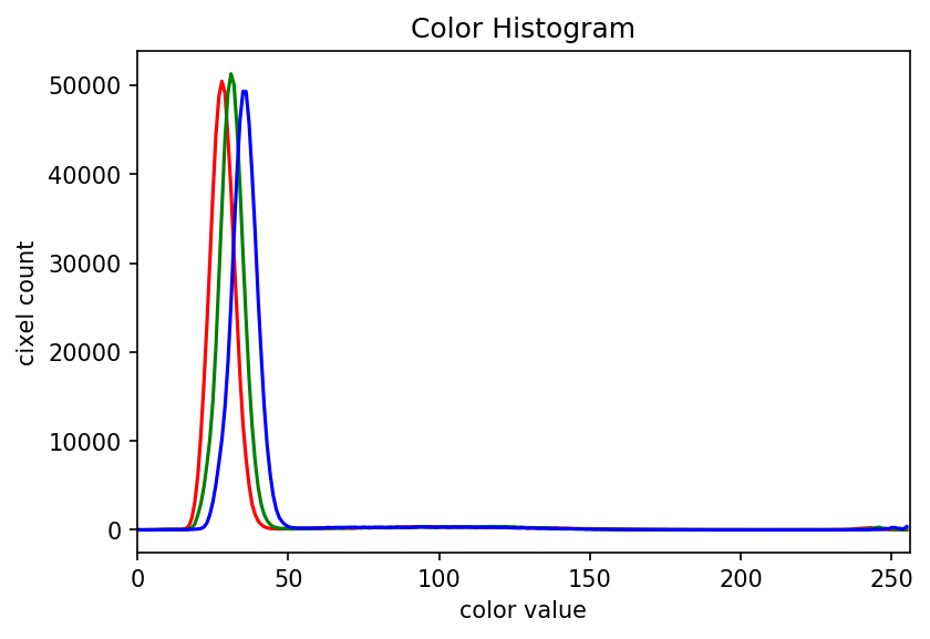
Color histogram with a mask (25 min)
We can also apply a mask to the images we apply the color histogram process to, in the same way we did for grayscale histograms. Consider this image of a well plate, where various chemical sensors have been applied to water and various concentrations of hydrochloric acid and sodium hydroxide:
Suppose we are interested in the color histogram of one of the sensors in the well plate image, specifically, the seventh well from the left in the topmost row, which shows Erythrosin B reacting with water.
Use ImageJ to find the center of that well and the radius (in pixels) of the well. Then, navigate to the Desktop/workshops/image-processing/05-creating-histograms directory, and edit the ColorHistogramMask.py program.
Guided by the comments in the ColorHistogramMask.py program, create a circular mask to select only the desired well. Then, use that mask to apply the color histogram operation to that well. When you execute the program on the plate-01.tif image, your program should display
maskedImg, which will look like this:
And, the program should produce a color histogram that looks like this:
Solution
Here is the modified version of ColorHistogramMask.py that produced the preceding images.
"""
 * Python program to create a color histogram on a masked image.
 *
 * Usage: python ColorHistogramMask.py <filename>
"""
import sys
import skimage.io
import skimage.viewer
import skimage.draw
import numpy as np
from matplotlib import pyplot as plt

# read original image, in full color, based on command
# line argument
image = skimage.io.imread(fname=sys.argv[1])

# display the original image
viewer = skimage.viewer.ImageViewer(image)
viewer.show()

# create a circular mask to select the 7th well in the first row
# WRITE YOUR CODE HERE
mask = np.zeros(shape=image.shape[0:2], dtype="bool")
circle = skimage.draw.circle(240, 1053, radius=49, shape=image.shape[:2])
mask[circle] = 1

# just for display:
# make a copy of the image, call it masked_image, and
# use np.logical_not() and indexing to apply the mask to it
# WRITE YOUR CODE HERE
masked_img = image[:]
masked_img[np.logical_not(mask)] = 0

# create a new window and display maskedImg, to verify the
# validity of your mask
# WRITE YOUR CODE HERE
viewer = skimage.viewer.ImageViewer(masked_img)
viewer.show()

# list to select colors of each channel line
colors = ("r", "g", "b")
channel_ids = (0, 1, 2)

# create the histogram plot, with three lines, one for
# each color
plt.xlim([0, 256])
for (channel_id, c) in zip(channel_ids, colors):
    # change this to use your circular mask to apply the histogram
    # operation to the 7th well of the first row
    # MODIFY CODE HERE
    histogram, bin_edges = np.histogram(
        image[:, :, channel_id][mask], bins=256, range=(0, 256)
    )

    plt.plot(histogram, color=c)

plt.xlabel("color value")
plt.ylabel("pixel count")

plt.show()
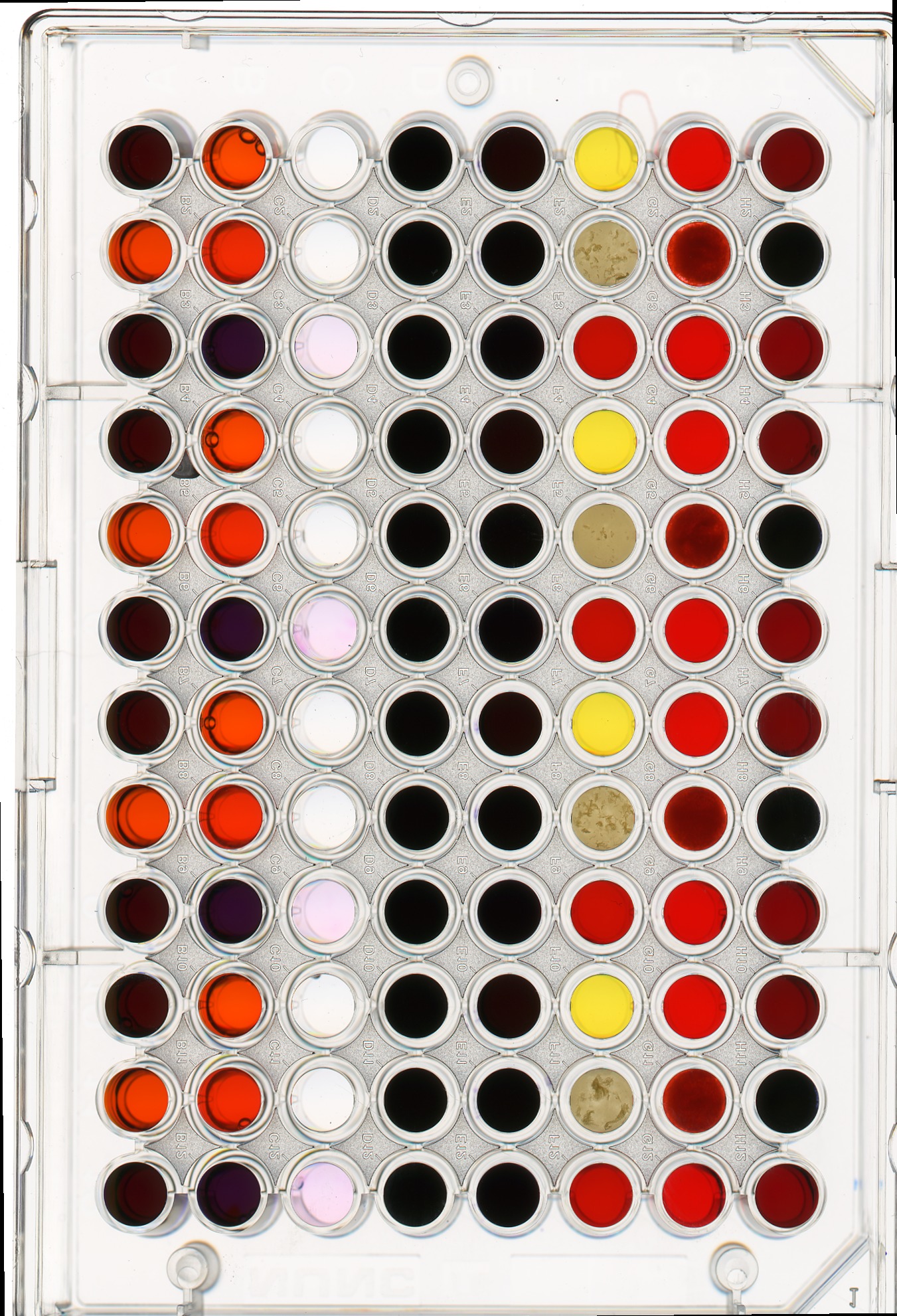
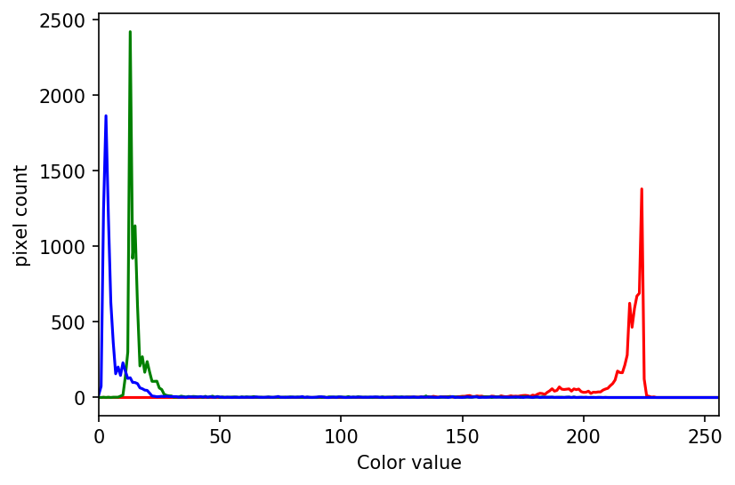
Histograms for the morphometrics challenge (10 min)
Using the grayscale and color histogram programs we developed in this episode, create histograms for the bacteria colonies in the Desktop/workshops/image-processing/10-challenges directory. Save the histograms for later use.
Key Points
We can load images in grayscale by passing the
as_gray=Trueparameter to theskimage.io.imread()function.We can create histograms of images with the
np.histogramfunction.We can separate the RGB channels of an image using slicing operations.
We can display histograms using the
matplotlib pyplotfigure(),title(),xlabel(),ylabel(),xlim(),plot(), andshow()functions.
Blurring images
Overview
Teaching: 10 min
Exercises: 40 minQuestions
How can we apply a low-pass blurring filter to an image?
Objectives
Explain why applying a low-pass blurring filter to an image is beneficial.
Apply a Gaussian blur filter to an image using skimage.
Explain what often happens if we pass unexpected values to a Python function.
In this episode, we will learn how to use skimage functions to blur images.
When we blur an image, we make the color transition from one side of an
edge in the image to another smooth rather than sudden. The effect is to
average out rapid changes in pixel intensity. The blur, or smoothing,
of an image removes “outlier” pixels that may be noise in the image. Blurring
is an example of applying a low-pass filter to an image. In computer vision,
the term “low-pass filter” applies to removing noise from an image while
leaving the majority of the image intact. A blur is a very common operation
we need to perform before other tasks such as edge detection. There are
several different blurring functions in the skimage.filters module, so we
will focus on just one here, the Gaussian blur.
Gaussian blur
Consider this image of a cat, in particular the area of the image outlined by the white square.
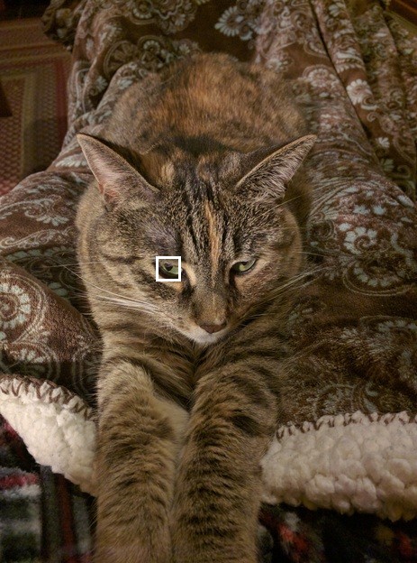
Now, zoom in on the area of the cat’s eye, as shown in the left-hand image below. When we apply a blur filter, we consider each pixel in the image, one at a time. In this example, the pixel we are applying the filter to is highlighted in red, as shown in the right-hand image.
![]()
In a blur, we consider a rectangular group of pixels surrounding the pixel to filter. This group of pixels, called the kernel, moves along with the pixel that is being filtered. So that the filter pixel is always in the center of the kernel, the width and height of the kernel must be odd. In the example shown above, the kernel is square, with a dimension of seven pixels.
To apply this filter to the current pixel, a weighted average of the the color values of the pixels in the kernel is calculated. In a Gaussian blur, the pixels nearest the center of the kernel are given more weight than those far away from the center. This averaging is done on a channel-by-channel basis, and the average channel values become the new value for the filtered pixel. Larger kernels have more values factored into the average, and this implies that a larger kernel will blur the image more than a smaller kernel.
To get an idea of how this works, consider this plot of the two-dimensional Gaussian function:
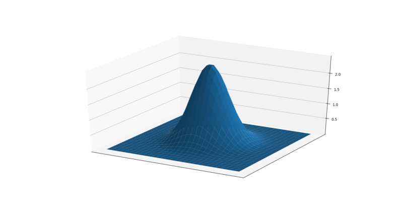
Imagine that plot overlaid over the kernel for the Gaussian blur filter. The height of the plot corresponds to the weight given to the underlying pixel in the kernel. I.e., the pixels close to the center become more important to the filtered pixel color than the pixels close to the edge of the kernel. The shape of the Gaussian function is controlled via its standard deviation, or sigma. A large sigma value results in a flatter shape, while a smaller sigma value results in a more pronounced peak. The mathematics involved in the Gaussian blur filter are not quite that simple, but this explanation gives you the basic idea.
To illustrate the blur process, consider the blue channel color values from the seven-by-seven kernel illustrated above:
68  82 71 62 100  98  61
90  67 74 78  91  85  77
50  53 78 82  72  95 100
87  89 83 86 100 116 128
89 108 86 78  92  75 100
90  83 89 73  68  29  18
77 102 70 57  30  30  50
The filter is going to determine the new blue channel value for the center pixel – the one that currently has the value 86. The filter calculates a weighted average of all the blue channel values in the kernel, {76, 83, 81, …, 39, 53, 68}, giving higher weight to the pixels near the center of the kernel. This weighted average would be the new value for the center pixel. The same process would be used to determine the green and red channel values, and then the kernel would be moved over to apply the filter to the next pixel in the image.
Something different needs to happen for pixels near the edge of the image, since the kernel for the filter may be partially off the image. For example, what happens when the filter is applied to the upper-left pixel of the image? Here are the blue channel pixel values for the upper-left pixel of the cat image, again assuming a seven-by-seven kernel:
  x   x   x   x   x   x   x
  x   x   x   x   x   x   x
  x   x   x   x   x   x   x
  x   x   x   4   5   9   2
  x   x   x   5   3   6   7
  x   x   x   6   5   7   8
  x   x   x   5   4   5   3
The upper-left pixel is the one with value 4. Since the pixel is at the upper-left corner. there are no pixels underneath much of the kernel; here, this is represented by x’s. So, what does the filter do in that situation?
The default mode is to fill in the nearest pixel value from the image. For each of the missing x’s the image value closest to the x is used. If we fill in a few of the missing pixels, you will see how this works:
  x   x   x   4   x   x   x
  x   x   x   4   x   x   x
  x   x   x   4   x   x   x
  4   4   4   4   5   9   2
  x   x   x   5   3   6   7
  x   x   x   6   5   7   8
  x   x   x   5   4   5   3
Another strategy to fill those missing values is to reflect the pixels that are in the image to fill in for the pixels that are missing from the kernel.
  x   x   x   5   x   x   x
  x   x   x   6   x   x   x
  x   x   x   5   x   x   x
  2   9   5   4   5   9   2
  x   x   x   5   3   6   7
  x   x   x   6   5   7   8
  x   x   x   5   4   5   3
A similar process would be used to fill in all of the other missing pixels from the kernel. Other border modes are available; you can learn more about them in the skimage documentation.
This animation shows how the blur kernel moves along in the original image in order to calculate the color channel values for the blurred image.
skimage has built-in functions to perform blurring for us, so we do not have to perform all of these mathematical operations ourselves. The following Python program shows how to use the skimage Gaussian blur function.
"""
 * Python script to demonstrate Gaussian blur.
 *
 * usage: python GaussBlur.py <filename> <sigma>
"""
import skimage
from skimage.viewer import ImageViewer
import sys

# get filename and kernel size from command line
filename = sys.argv[1]
sigma = float(sys.argv[2])
In this case, the program takes two command-line parameters. The first is the filename of the image to filter, and the second is the sigma of the Gaussian.
In the program, we first import the required libraries, as we have done before. Then, we read the two command-line arguments. The first, the filename, should be familiar code by now. For the sigma argument, we have to convert the second argument from a string, which is how all arguments are read into the program, into a float, which is what we will use for our sigma. This is done with the
sigma = float(sys.argv[2])
line of code. The float() function takes a string as its parameter, and returns
the floating point number equivalent.
What happens if the
float()parameter does not look like a number? (10 min)In the program fragment, we are using the
float()function to parse the second command-line argument, which comes in to the program as a string, and convert it into an integer. What happens if the second command-line argument does not look like an integer? Let us perform an experiment to find out.Write a simple Python program to read one command-line argument, convert the argument to an integer, and then print out the result. Then, run your program with an integer argument, and then again with some non-integer arguments. For example, if your program is named float_arg.py, you might perform these runs:
python float_arg.py 3.14159
python float_arg.py puppy
python float_arg.py 13
What does
float()do if it receives a string that cannot be parsed into an integer?Solution
Here is a simple program to read in one command-line argument, parse it as and integer, and print out the result:
"""
 * Read a command-line argument, parse it as an integer, and
 * print out the result.
 *
 * usage: python float_arg.py <argument>
"""
import sys

value = float(sys.argv[1])
print("Your command-line argument is:", value)
Executing this program with the three command-line arguments suggested above produces this output:
Your command-line argument is: 3.14159

Traceback (most recent call last):
  File "float_arg.py", line 9, in <module>
    value = float(sys.argv[1])
ValueError: could not convert string to float: 'puppy'

Your command-line argument is: 13.0
You can see that if we pass in an invalid value to the
float()function, the Python interpreter halts the program and prints out an error message, describing what the problem was.
Next, the program reads and displays the original, unblurred image. This should also be very familiar to you at this point.
# read and display original image
image = skimage.io.imread(fname=filename)
viewer = ImageViewer(image)
viewer.show()
Now we apply the average blur:
# apply Gaussian blur, creating a new image
blurred = skimage.filters.gaussian(
    image, sigma=(sigma, sigma), truncate=3.5, multichannel=True)
The first two parameters to skimage.filters.gaussian() are the image to blur,
image, and a tuple defining the sigma to use in y- and x-direction,
(sigma, sigma). The third parameter truncate gives the radius of the kernel
in terms of sigmas. A Gaussian is defined from -infinity to +infinity. A
discrete Gaussian can only approximate the real function. The truncate
parameter steers at what distance to the center of the function it is not
approximated any more. In the above example we set truncate to 3.5. With a
sigma of 1.0 the resulting kernel size would be 7.
The default value for truncate in sklearn is 4.0.
The last parameter is to tell skimage how to interpret our image, that has three
dimensions, as a multichannel color image.
After the blur filter has been executed, the program wraps things up by
displaying the blurred image in a new window.
# display blurred image
viewer = ImageViewer(blurred)
viewer.show()
Here is a constructed image to use as the input for the preceding program.
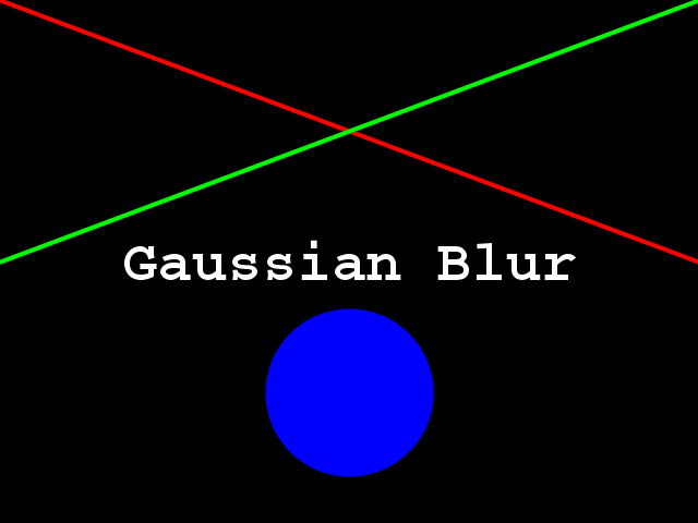
When the program runs, it displays the original image, applies the filter, and then shows the blurred result. The following image is the result after applying a filter with a sigma of 3.0.
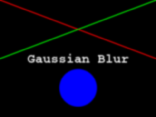
Experimenting with sigma values (5 min)
Navigate to the Desktop/workshops/image-processing/06-blurring directory and execute the GaussBlur.py script, which contains the program shown above. Execute it with two command-line parameters, like this:
python GaussBlur.py GaussianTarget.png 1.0Remember that the first command-line argument is the name of the file to filter, and the second is the sigma value. Now, experiment with the sigma value, running the program with smaller and larger values. Generally speaking, what effect does the sigma value have on the blurred image?
Solution
Generally speaking, the larger the sigma value, the more blurry the result. A larger sigma will tend to get rid of more noise in the image, which will help for other operations we will cover soon, such as edge detection. However, a larger sigma also tends to eliminate some of the detail from the image. So, we must strike a balance with the sigma value used for blur filters.
Experimenting with kernel shape (10 min)
Now, modify the GaussBlur.py program so that it takes three command-line parameters instead of two. The first parameter should still be the name of the file to filter. The second and third parameters should be the sigma values in y- and x-direction for the Gaussian to use, so that the resulting kernel is rectangular instead of square. The new version of the program should be invoked like this:
python GaussBlur.py GaussianTarget.png 1.0 2.0Using the program like this utilizes a Gaussian with a sigma of 1.0 in y- direction and 2.0 in x-direction for blurring
Solution
"""
 * Python script to demonstrate Gaussian blur.
 *
 * usage: python GaussBlur.py <filename> <sigma_y> <sigma_x>
"""
import skimage
from skimage.viewer import ImageViewer
import sys

# get filename and kernel size from command line
filename = sys.argv[1]
sigma_y = float(sys.argv[2])
sigma_x = float(sys.argv[3])

# read and display original image
image = skimage.io.imread(fname=filename)
viewer = ImageViewer(image)
viewer.show()

# apply Gaussian blur, creating a new image
blurred = skimage.filters.gaussian(
    image, sigma=(sigma_y, sigma_x), truncate=3.5, multichannel=True
)

# display blurred image
viewer = ImageViewer(blurred)
viewer.show()
Other methods of blurring
The Gaussian blur is a way to apply a low-pass filter in skimage. It is often
used to remove Gaussian (i. e., random) noise from the image.
For other kinds of noise, e.g. “salt and pepper” or “static” noise, a
median filter is typically used.
See the skimage.filter documentation
for a list of available filters.
Blurring the bacteria colony images (15 min)
As we move further into the workshop, we will see that in order to complete the colony-counting morphometric challenge at the end, we will need to read the bacteria colony images as grayscale, and blur them, before moving on to the tasks of actually counting the colonies. Create a Python program to read one of the colony images (with the filename provided as a command-line parameter) as grayscale, and then apply a Gaussian blur to the image. You should also provide the sigma for the blur as a second command-line parameter. Do not alter the original image. As a reminder, the images are located in the Desktop/workshops/image-processing/10-challenges/morphometrics directory.
Key Points
Applying a low-pass blurring filter smooths edges and removes noise from an image.
Blurring is often used as a first step before we perform Thresholding, Edge Detection, or before we find the Contours of an image.
The Gaussian blur can be applied to an image with the
skimage.filters.gaussian()function.Larger sigma values may remove more noise, but they will also remove detail from an image.
The
float()function can be used to parse a string into an float.
Thresholding
Overview
Teaching: 30 min
Exercises: 65 minQuestions
How can we use thresholding to produce a binary image?
Objectives
Explain what thresholding is and how it can be used.
Use histograms to determine appropriate threshold values to use for the thresholding process.
Apply simple, fixed-level binary thresholding to an image.
Explain the difference between using the operator
>or the operator<to threshold an image represented by a numpy array.Describe the shape of a binary image produced by thresholding via
>or<.Explain when Otsu’s method of adaptive thresholding is appropriate.
Apply adaptive thresholding to an image using Otsu’s method.
Use the
np.nonzero()function to count the number of non-zero pixels in an image.
In this episode, we will learn how to use skimage functions to apply thresholding to an image. Thresholding is a type of image segmentation, where we change the pixels of an image to make the image easier to analyze. In thresholding, we convert an image from color or grayscale into a binary image, i.e., one that is simply black and white. Most frequently, we use thresholding as a way to select areas of interest of an image, while ignoring the parts we are not concerned with. We have already done some simple thresholding, in the “Manipulating pixels” section of the Skimage Images episode. In that case, we used a simple NumPy array manipulation to separate the pixels belonging to the root system of a plant from the black background. In this episode, we will learn how to use skimage functions to perform thresholding. Then, we will use the masks returned by these functions to select the parts of an image we are interested in.
Simple thresholding
Consider this image, with a series of crudely cut shapes set against a white background. The black outline around the image is not part of the image.

Now suppose we want to select only the shapes from the image. In other words,
we want to leave the pixels belonging to the shapes “on,” while turning the
rest of the pixels “off,” by setting their color channel values to zeros. The
skimage library has several different methods of thresholding. We will start
with the simplest version, which involves an important step of human
input. Specifically, in this simple, fixed-level thresholding, we have to
provide a threshold value, t.
The process works like this. First, we will load the original image, convert
it to grayscale, and blur it with one of the methods from the
Blurring episode. Then, we will use the
> operator to apply the threshold t, a number in the closed range [0.0, 1.0].
Pixels with color values on one
side of t will be turned “on,” while pixels with color values on the other side
will be turned “off.” In order to use this function, we have to determine a good
value for t. How might we do that? Well, one way is to look at a grayscale
histogram of the image. Here is the histogram produced by the
GrayscaleHistogram.py program from the
Creating Histograms episode, if we
run it on the colored shapes image shown above.
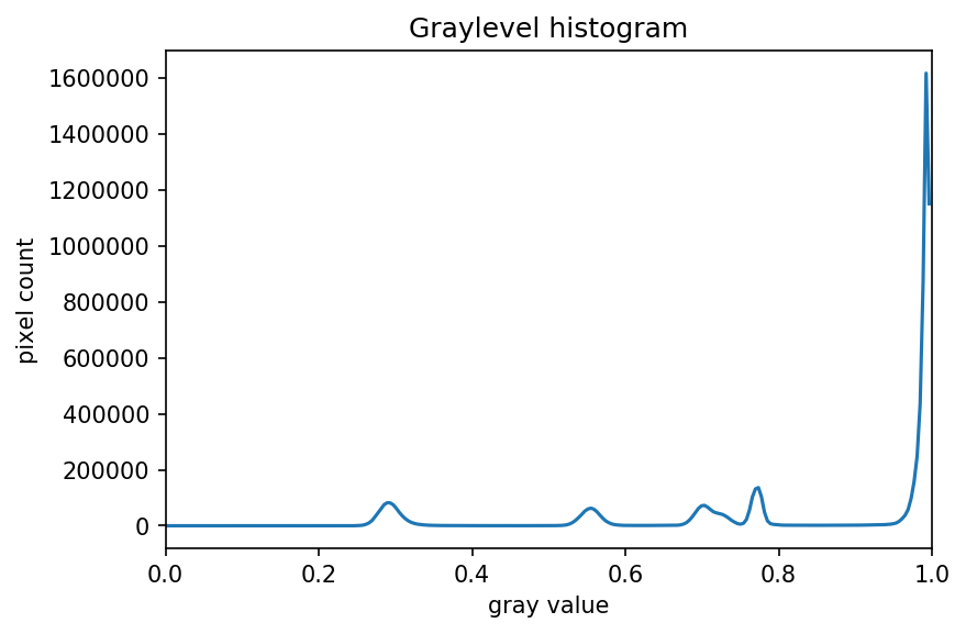
Since the image has a white background, most of the pixels in the image are
white. This corresponds nicely to what we see in the histogram: there is a
spike near the value of 1.0. If we want to select the shapes and not the
background, we want to turn off the white background pixels, while leaving the
pixels for the shapes turned on. So, we should choose a value of t somewhere
before the large peak and turn pixels above that value “off”.
Here are the first few lines of a Python program to apply simple thresholding to the image, to accomplish this task.
"""
 * Python script to demonstrate simple thresholding.
 *
 * usage: python Threshold.py <filename> <sigma> <threshold>
"""
import sys
import numpy as np
import skimage.color
import skimage.filters
import skimage.io
import skimage.viewer

# get filename, sigma, and threshold value from command line
filename = sys.argv[1]
sigma = float(sys.argv[2])
t = float(sys.argv[3])

# read and display the original image
image = skimage.io.imread(fname=filename)
viewer = skimage.viewer.ImageViewer(image)
viewer.show()
This program takes three command-line arguments: the filename of the image to
manipulate, the sigma of the Gaussian used during the blurring step (which, if you recall
from the Blurring episode, must be a float),
and finally, the threshold value t, which should be a float in the closed
range [0.0, 1.0]. The program takes the command-line values and stores them in
variables named filename, sigma, and t, respectively.
Next, the program reads the original image based on the filename value, and
displays it.
Now is where the main work of the program takes place.
# blur and grayscale before thresholding
blur = skimage.color.rgb2gray(image)
blur = skimage.filters.gaussian(blur, sigma=k)
First, we convert the
image to grayscale and then blur it, using the skimage.filter.gaussian() function we
learned about in the Blurring episode.
We convert the input image to grayscale for easier thresholding.
The fixed-level thresholding is performed using numpy comparison operators.
# perform inverse binary thresholding
mask = blur < t_rescaled
Here, we want to turn “on” all pixels which have values smaller than the threshold,
so we use the less operator < to compare the blurred image blur to the threshold t.
The operator returns a binary image, that we capture in the variable mask.
It has only one channel, and each of its values is either 0 or 1. Here is a
visualization of the binary image created by the thresholding operation.
The program used parameters of sigma = 2 and t = 0.8 to produce this image. You can
see that the areas where the shapes were in the original area are now white,
while the rest of the mask image is black.
We can now apply the mask to the original colored image as we have learned in the Drawing and Bitwise Operations episode.
# use the mask to select the "interesting" part of the image
sel = np.zeros_like(image)
sel[mask] = image[mask]

# display the result
viewer = skimage.viewer.ImageViewer(sel)
viewer.view()
What we are left with is only the colored shapes from the original, as shown in this image:
More practice with simple thresholding (15 min)
Now, it is your turn to practice. Suppose we want to use simple thresholding to select only the colored shapes from this image:
First, use the GrayscaleHistogram.py program in the Desktop/workshops/image-processing/05-creating-histograms directory to examine the grayscale histogram of the more-junk.jpg image, which you will find in the Desktop/workshops/image-processing/07-thresholding directory. Via the histogram, what do you think would be a good value for the threshold value,
t?Solution
Here is the histogram for the more-junk.jpg image.
We can see a large spike around 0.3, and a smaller spike around 0.7. The spike near 0.3 represents the darker background, so it seems like a
tvalue close to 0.5 would be a good choice.Now, modify the ThresholdPractice.py program in the Desktop/workshops/image-processing/07-thresholding directory to turn the pixels above the
tvalue on and turn the pixels below thetvalue off. To do this, change the comparison operator less<to greater>. Then execute the program on the more-junk.jpg image, using a reasonable value for k and thetvalue you obtained from the histogram. If everything works as it should, your output should show only the colored shapes on a pure black background.Solution
Here is the modified ThresholdPractice.py program.
"""
 * Python script to practice simple thresholding.
 *
 * usage: python ThresholdPractice.py <filename> <sigma> <threshold>
"""
import sys
import numpy as np
import skimage.color
import skimage.fiters
import skimage.io
import skimage.viewer

# get filename, sigma, and threshold value from command line
filename = sys.argv[1]
sigma = float(sys.argv[2])
t = float(sys.argv[3])

# read and display the original image
image = skimage.io.imread(fname=filename)
viewer = skimage.viewer.ImageViewer(image)
viewer.show()

# blur and grayscale before thresholding
blur = skimage.color.rgb2gray(image)
blur = skimage.filters.gaussian(blur, sigma=sigma)

# perform binary thresholding
# MODIFY CODE HERE!
mask = blur > t

# display the mask image
viewer = skimage.viewer.ImageViewer(mask)
viewer.show()

# use the mask to select the "interesting" part of the image
sel = np.zeros_like(image)
sel[mask] = image[mask]

# display the result
viewer = skimage.viewer.ImageViewer(sel)
viewer.show()
Using a Gaussian with sigma = 2 and threshold t = 0.5, we obtain this mask:
And applying the mask results in this selection of shapes:
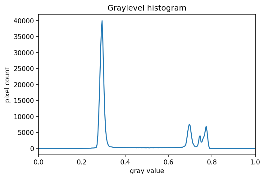


Adaptive thresholding
There are also skimage methods to perform adaptive thresholding. The chief advantage of adaptive thresholding is that the value of the threshold, t, is determined automatically for us. One such method, Otsu’s method, is particularly useful for situations where the grayscale histogram of an image has two peaks. Consider this maize root system image, which we have seen before in the Skimage Images episode.
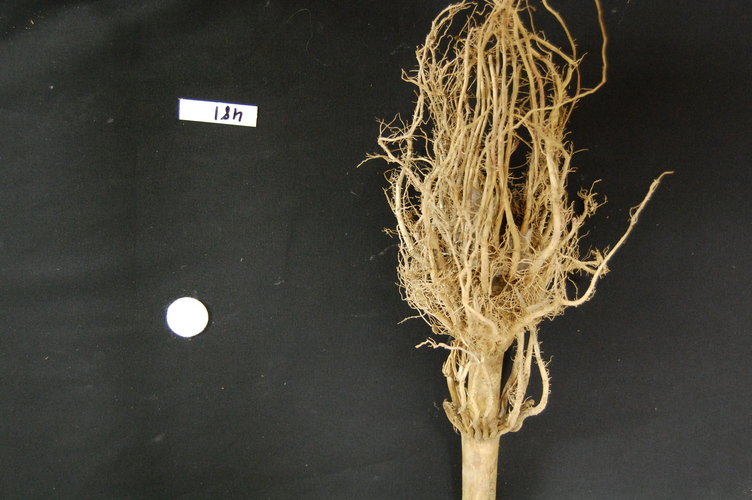
Now, look at the grayscale histogram of this image, as produced by our GrayscaleHistogram.py program from the Creating Histograms episode.

The histogram has a significant peak around 0.2, and a second, albeit smaller peak very near 1.0. Thus, this image is a good candidate for thresholding with Otsu’s method. The mathematical details of how this work are complicated (see the skimage documentation if you are interested), but the outcome is that Otsu’s method finds a threshold value between the two peaks of a grayscale histogram.
The skimage.filters.threshold_otsu() function can be used to determine
the adaptive threshold via Otsu’s method. Then numpy comparison operators can be
used to apply it as before.
Here is a Python program illustrating how to perform thresholding with Otsu’s
method using the skimage.filters.threshold_otsu function. We start by reading and displaying
the target image.
"""
 * Python script to demonstrate adaptive thresholding using Otsu's method.
 *
 * usage: python AdaptiveThreshold.py <filename> <sigma>
"""
import sys
import numpy as np
import skimage.color
import skimage.filters
import skimage.io
import skimage.viewer

# get filename and sigma value from command line
filename = sys.argv[1]
sigma = float(sys.argv[2])

# read and display the original image
image = skimage.io.imread(fname=filename)
viewer = skimage.viewer.ImageViewer(image)
viewer.show()
The program begins with the now-familiar imports and command line parameters.
Here we only have to get the filename and the sigma of the Gaussian kernel from the command
line, since Otsu’s method will automatically determine the thresholding value
t. Then, the original image is read and displayed.
Next, a blurred grayscale image is created.
# blur and grayscale before thresholding
blur = skimage.color.rgb2gray(image)
blur = skimage.filters.gaussian(image, sigma=sigma)
We determine the threshold via the skimage.filters.threshold_otsu() function:
# perform adaptive thresholding
t = skimage.filters.threshold_otsu(blur)
mask = blur > t
The function skimage.filters.threshold_otsu() uses Otsu’s method to automatically
determine the threshold value based on its inputs grayscale histogram and returns it.
Then, we use the comparison operator > for binary thesholding. As we have seen before,
pixels above the threshold value will be turned on, those below the threshold will be turned off.
For this root image, and a Gaussian blur with a sigma of 1.0, the computed threshold value is 0.42, and the resulting mask is:
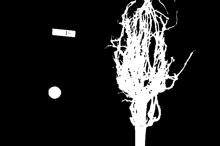
Next, we display the mask and use it to select the foreground
viewer = skimage.viewer.ImageViewer(mask)
viewer.show()

# use the mask to select the "interesting" part of the image
sel = np.zeros_like(image)
sel[mask] = image[mask]

# display the result
viewer = skimage.viewer.ImageViewer(sel)
viewer.show()
Here is the result:
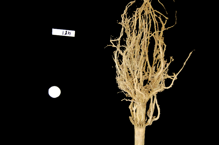
Application: measuring root mass
Let us now turn to an application where we can apply thresholding and other techniques we have learned to this point. Consider these four maize root system images.

Now suppose we are interested in the amount of plant material in each image, and in particular how that amount changes from image to image. Perhaps the images represent the growth of the plant over time, or perhaps the images show four different maize varieties at the same phase of their growth. In any case, the question we would like to answer is, “how much root mass is in each image?” We will construct a Python program to measure this value for a single image, and then create a Bash script to execute the program on each trial image in turn.
Our strategy will be this:
- Read the image, converting it to grayscale as it is read. For this application we do not need the color image.
- Blur the image.
- Use Otsu’s method of thresholding to create a binary image, where the pixels that were part of the maize plant are white, and everything else is black.
- Save the binary image so it can be examined later.
- Count the white pixels in the binary image, and divide by the number of pixels in the image. This ratio will be a measure of the root mass of the plant in the image.
- Output the name of the image processed and the root mass ratio.
Here is a Python program to implement this root-mass-measuring strategy. Almost all of the code should be familiar, and in fact, it may seem simpler than the code we have worked on thus far, because we are not displaying any of the images with this program. Our program here is intended to run and produce its numeric result – a measure of the root mass in the image – without human intervention.
"""
 * Python program to determine root mass, as a ratio of pixels in the
 * root system to the number of pixels in the entire image.
 *
 * usage: python RootMass.py <filename> <sigma>
"""
import sys
import numpy as np
import skimage.io
import skimage.filters


# get filename and sigma value from command line
filename = sys.argv[1]
sigma = float(sys.argv[2])

# read the original image, converting to grayscale
img = skimage.io.imread(fname=filename, as_gray=True)
The program begins with the usual imports and reading of command-line parameters. Then, we read the original image, based on the filename parameter, in grayscale.
Next the grayscale image is blurred with a Gaussian that is defined by the sigma parameter.
# blur before thresholding
blur = skimage.filters.gaussian(img, sigma=sigma)
Following that, we create a binary image with Otsu’s method for thresholding, just as we did in the previous section. Since the program is intended to produce numeric output, without a person shepherding it, it does not display any of the images.
# perform adaptive thresholding to produce a binary image
t = skimage.filters.threshold_otsu(blur)
binary = blur > t
We do, however, want to save the binary images, in case we wish to examine them at a later time. That is what this block of code does:
# save binary image; first find beginning of file extension
dot = filename.index(".")
binary_file_name = filename[:dot] + "-binary" + filename[dot:]
skimage.io.imsave(fname=binary_file_name, arr=skimage.img_as_ubyte(binary))
This code does a little bit of string manipulation to determine the filename
to use when the binary image is saved. For example, if the input filename being
processed is trial-020.jpg, we want to save the corresponding binary image
as trial-020-binary.jpg. To do that, we first determine the index of the
dot between the filename and extension – and note that we assume that there is
only one dot in the filename! Once we have the location of the dot, we can use
slicing to pull apart the filename string, inserting “-binary” in between the
end of the original name and the extension. Then, the binary image is saved via
a call to the skimage.io.imsave() function.
In order to convert from the binary range of 0 and 1 of the mask to a gray level image that can be saved as png, we use the skimage.img_as_ubyte utility function.
Finally, we can examine the code that is the reason this program exists! This block of code determines the root mass ratio in the image:
# determine root mass ratio
rootPixels = np.nonzero(binary)
w = binary.shape[1]
h = binary.shape[0]
density = rootPixels / (w * h)

# output in format suitable for .csv
print(filename, density, sep=",")
Recall that we are working with a binary image at this point; every pixel in
the image is either zero (black) or 1 (white). We want to count the number
of white pixels, which is easily accomplished with a call to the
np.count_nonzero function. Then we determine the width and height of the
image, via the first and second elements of the image’s shape. Then the
density ratio is calculated by dividing the number of white pixels by the
total number of pixels in the image. Then, the program prints out the
name of the file processed and the corresponding root density.
If we run the program on the trial-016.jpg image, with a sigma value of 1.5, we would execute the program this way:
python RootMass.py trial-016.jpg 1.5
and the output we would see would be this:
trial-016.jpg,0.0482436835106383
We have four images to process in this example, and in a real-world scientific situation, there might be dozens, hundreds, or even thousands of images to process. To save us the tedium of running the Python program on each image, we can construct a Bash shell script to run the program multiple times for us. Here is a sample script, which assumes that the images all start with the trial- prefix and end with the .jpg file extension. The script also assumes that the images, the RootMass.py program, and the script itself are all in the same directory.
#!/bin/bash
# Run the root density mass on all of the root system trail images.

# first, remove existing binary output images
rm *-binary.jpg

# then, execute the program on all the trail images
for f in trial-*.jpg
do
	python RootMass.py $f 1.5
done
The script begins by deleting any prior versions of the binary images. After
that, the script uses a for loop to iterate through all of the input images,
and execute the RootMass.py on each image with a sigma of 1.5.
When we execute the script from the command line, we will see output like this:
trial-016.jpg,0.0482436835106383
trial-020.jpg,0.06346941489361702
trial-216.jpg,0.14073969414893617
trial-293.jpg,0.13607895611702128
It would probably be wise to save the output of our multiple runs to a file that we can analyze later on. We can do that very easily by redirecting the output stream that would normally appear on the screen to a file. Assuming the shell script is named rootmass.sh, this would do the trick:
bash rootmass.sh > rootmass.csv
Ignoring more of the images – brainstorming (10 min)
Let us take a closer look at the binary images produced by the proceeding program.
Our root mass ratios include white pixels that are not part of the plant in the image, do they not? The numbered labels and the white circles in each image are preserved during the thresholding, and therefore their pixels are included in our calculations. Those extra pixels might have a slight impact on our root mass ratios, especially the labels, since the labels are not the same size in each image. How might we remove the labels and circles before calculating the ratio, so that our results are more accurate? Brainstorm and think about some options, given what we have learned so far.
Solution
One approach we might take is to try to completely mask out a region from each image, particularly, the area containing the white circle and the numbered label. If we had coordinates for a rectangular area on the image that contained the circle and the label, we could mask the area out easily by using techniques we learned in the Drawing and Bitwise Operations episode.
However, a closer inspection of the binary images raises some issues with that approach. Since the roots are not always constrained to a certain area in the image, and since the circles and labels are in different locations each time, we would have difficulties coming up with a single rectangle that would work for every image. We could create a different masking rectangle for each image, but that is not a practicable approach if we have hundreds or thousands of images to process.
Another approach we could take is to apply two thresholding steps to the image. First, we could use simple binary thresholding to select and remove the white circle and label from the image, and then use Otsu’s method to turn on the pixels in the plant portion of the image.

Ignoring more of the images – implementation (30 min)
Navigate to the Desktop/workshops/image-processing/07-thresholding directory, and edit the RootMassImproved.py program. This is a copy of the RootMass.py program developed above. Modify the program to apply simple inverse binary thresholding to remove the white circle and label from the image before applying Otsu’s method. Comments in the program show you where you should make your changes.
Solution
Here is how we can apply an initial round of thresholding to remove the label and circle from the image.
"""
 * Python program to determine root mass, as a ratio of pixels in the
 * root system to the number of pixels in the entire image.
 *
 * This version applies thresholding twice, to get rid of the white
 * circle and label from the image before performing the root mass
 * ratio calculations.
 *
 * usage: python RootMassImproved.py <filename> <sigma>
"""
import sys
import skimage.io
import skimage.filters

# get filename and sigma value from command line
filename = sys.argv[1]
sigma = float(sys.argv[2])

# read the original image, converting to grayscale
image = skimage.io.imread(fname=filename, as_gray=True)

# blur before thresholding
blur = skimage.filters.gaussian(img, sigma=sigma)

# WRITE CODE HERE
# perform binary thresholding to create a mask that selects
# the white circle and label, so we can remove it later
mask = blur > 0.95

# WRITE CODE HERE
# use the mask you just created to remove the circle and label from the
# blur image
blur[mask] = 0

# perform adaptive thresholding to produce a binary image
t = skimage.filters.threshold_otsu(blur)
binary = blur > t

# save binary image; first find extension beginning
dot = filename.index(".")
binary_file_name = filename[:dot] + "-binary" + filename[dot:]
skimage.io.imsave(fname=binary_file_name, arr=binary)

# determine root mass ratio
rootPixels = np.nonzero(binary)
w = binary.shape[1]
h = binary.shape[0]
density = float(rootPixels) / (w * h)

# output in format suitable for .csv
print(filename, density, sep=",")
Here are the binary images produced by this program. We have not completely removed the offending white pixels. Outlines still remain. However, we have reduced the number of extraneous pixels, which should make the output more accurate.
The output of the improved program does illustrate that the white circles and labels were skewing our root mass ratios:
trial-016.jpg,0.045935837765957444
trial-020.jpg,0.058800033244680854
trial-216.jpg,0.13705003324468085
trial-293.jpg,0.13164461436170213
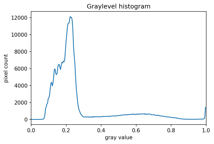
Thresholding a bacteria colony image (10 min)
In the Desktop/workshops/image-processing/07-thresholding directory, you will find an image named colonies01.tif; this is one of the images you will be working with in the morphometric challenge at the end of the workshop. First, create a grayscale histogram of the image, and determine a threshold value for the image. Then, write a Python program to threshold a grayscale version of the image, leaving the pixels in the bacteria colonies “on,” while turning the rest of the pixels in the image “off.”
Key Points
Thresholding produces a binary image, where all pixels with intensities above (or below) a threshold value are turned on, while all other pixels are turned off.
The binary images produced by thresholding are held in two-dimensional NumPy arrays, since they have only one color value channel. They are boolean, hence they contain the values 0 (off) and 1 (on).
Thresholding can be used to create masks that select only the interesting parts of an image, or as the first step before Edge Detection or finding Contours.
Edge Detection
Overview
Teaching: 20 min
Exercises: 45 minQuestions
How can we automatically detect the edges of the objects in an image?
Objectives
Apply Canny edge detection to an image.
Explain how we can use sliders to expedite finding appropriate parameter values for our skimage function calls.
Create skimage windows with sliders and associated callback functions.
In this episode, we will learn how to use skimage functions to apply edge detection to an image. In edge detection, we find the boundaries or edges of objects in an image, by determining where the brightness of the image changes dramatically. Edge detection can be used to extract the structure of objects in an image. If we are interested in the number, size, shape, or relative location of objects in an image, edge detection allows us to focus on the parts of the image most helpful, while ignoring parts of the image that will not help us.
For example, once we have found the edges of the objects in the image (or once we have converted the image to binary using thresholding), we can use that information to find the image contours, which we will learn about in the following connected components episode. With the contours, we can do things like counting the number of objects in the image, measure the size of the objects, classify the shapes of the objects, and so on.
As was the case for blurring and thresholding, there are several different methods in skimage that can be used for edge detection, so we will examine only one in detail.
Introduction to edge detection
To begin our introduction to edge detection, let us look at an image with a very simple edge – this grayscale image of two overlapped pieces of paper, one black and and one white:
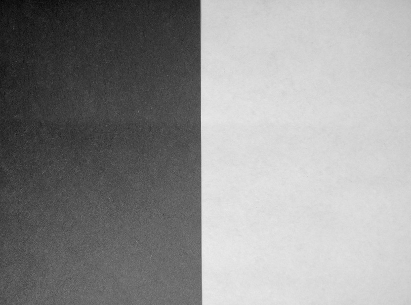
The obvious edge in the image is the vertical line between the black paper and the white paper. To our eyes, there is a quite sudden change between the black pixels and the white pixels. But, at a pixel-by-pixel level, is the transition really that sudden?
If we zoom in on the edge more closely, as in this image, we can see that the edge between the black and white areas of the image is not a clear-cut line.
![]()
We can learn more about the edge by examining the color values of some of the pixels. Imagine a short line segment, halfway down the image and straddling the edge between the black and white paper. This plot shows the pixel values (between 0 and 255, since this is a grayscale image) for forty pixels spanning the transition from black to white.
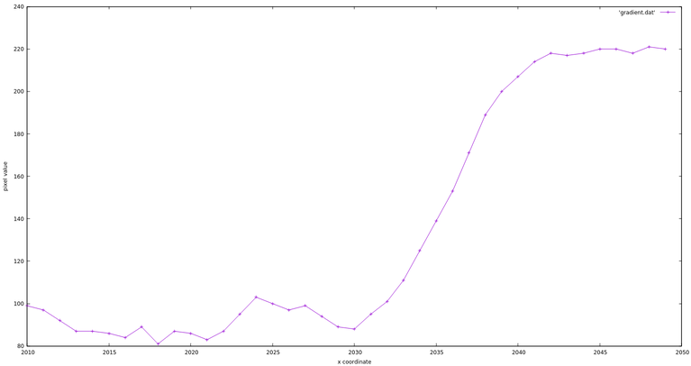
It is obvious that the “edge” here is not so sudden! So, any skimage method to detect edges in an image must be able to decide where the edge is, and place appropriately-colored pixels in that location.
Canny edge detection
Our edge detection method in this workshop is Canny edge detection, created
by John Canny in 1986. This method uses a series of steps, some incorporating
other types of edge detection. The skimage skimage.feature.canny() function performs
the following steps:
- A Gaussian blur (that is characterized by the
sigmaparameter, see introduction) is applied to remove noise from the image. (So if we are doing edge detection via this function, we should not perform our own blurring step.) - Sobel edge detection is performed on both the x and y dimensions, to find the intensity gradients of the edges in the image. Sobel edge detection computes the derivative of a curve fitting the gradient between light and dark areas in an image, and then finds the peak of the derivative, which is interpreted as the location of an edge pixel.
- Pixels that would be highlighted, but seem too far from any edge, are removed. This is called non-maximum suppression, and the result is edge lines that are thinner than those produced by other methods.
- A double threshold is applied to determine potential edges. Here extraneous pixels caused by noise or milder color variation than desired are eliminated. If a pixel’s gradient value – based on the Sobel differential – is above the high threshold value, it is considered a strong candidate for an edge. If the gradient is below the low threshold value, it is turned off. If the gradient is in between, the pixel is considered a weak candidate for an edge pixel.
- Final detection of edges is performed using hysteresis. Here, weak candidate pixels are examined, and if they are connected to strong candidate pixels, they are considered to be edge pixels; the remaining, non-connected weak candidates are turned off.
For a user of the skimage.feature.canny() edge detection function, there are three important
parameters to pass in: sigma for the Gaussian filter in step one and the low and high threshold values used in step four
of the process. These values generally are determined empirically, based on the
contents of the image(s) to be processed.
The following program illustrates how the skimage.feature.canny() method can be used to
detect the edges in an image.
We will execute the program on this image, which we used before in the Thresholding episode:
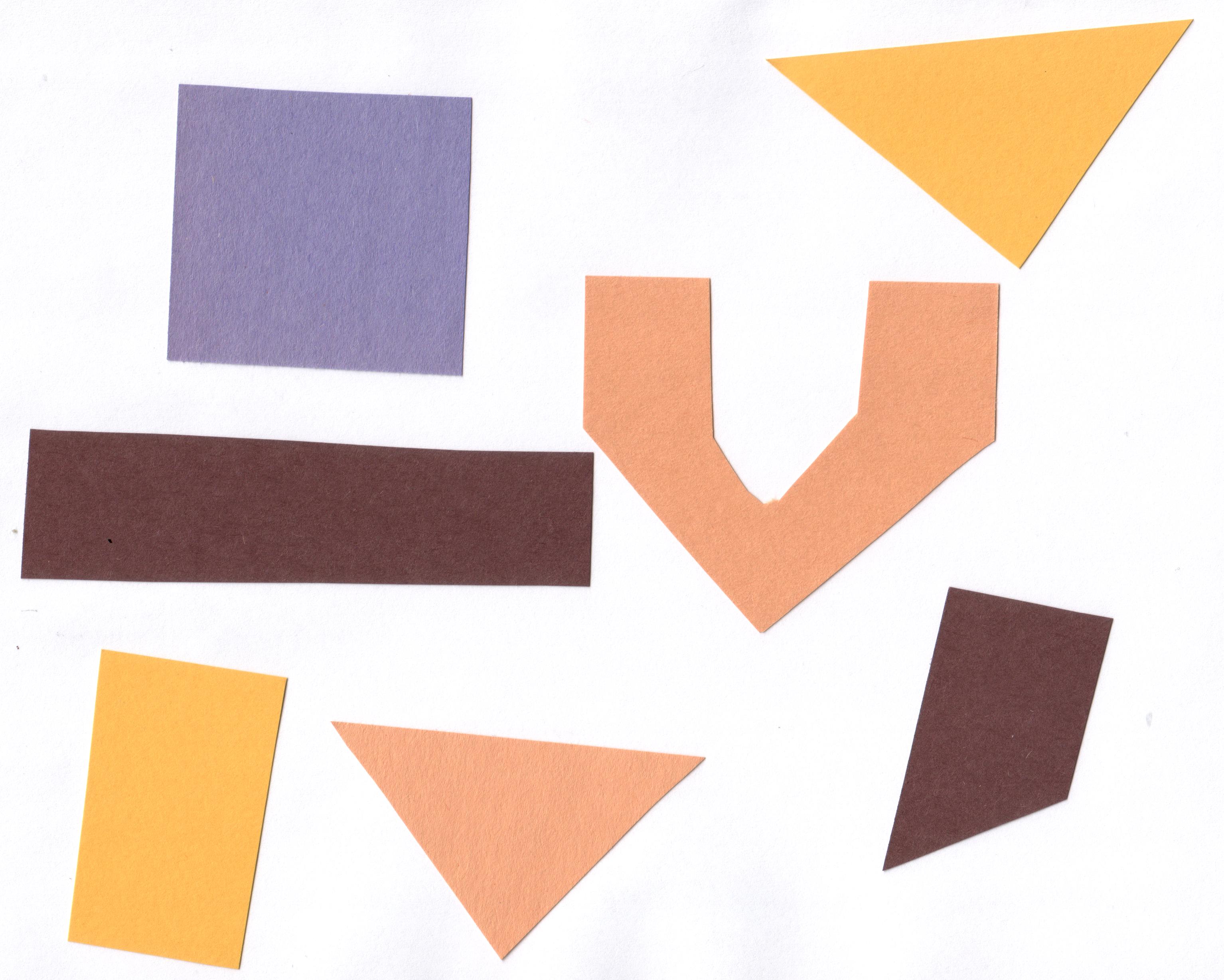
We are interested in finding the edges of the shapes in the image, and so the
colors are not important. Our strategy will be to read the image as grayscale,
and then apply Canny edge detection.
Note that when reading the image with skimage.io.imread(..., as_gray=True) the image is converted to a float64 grayscale with the original dtype range being mapped to values ranging from 0.0 to 1.0.
This program takes three command-line arguments: the filename of the image to process, and then two arguments related to the double thresholding in step four of the Canny edge detection process. These are the low and high threshold values for that step. After the required libraries are imported, the program reads the command-line arguments and saves them in their respective variables.
"""
 * Python script to demonstrate Canny edge detection.
 *
 * usage: python CannyEdge.py <filename> <sigma> <low_threshold> <high_threshold>
"""
import skimage
import skimage.feature
import skimage.viewer
import sys

# read command-line arguments
filename = sys.argv[1]
sigma = float(sys.argv[2])
low_threshold = float(sys.argv[3])
high_threshold = float(sys.argv[4])
Next, the original images is read, in grayscale, and displayed.
# load and display original image as grayscale
image = skimage.io.imread(fname=filename, as_gray=True)
viewer = skimage.viewer(image=image)
viewer.show()
Then, we apply Canny edge detection with this function call:
edges = skimage.feature.canny(
    image=image,
    sigma=sigma,
    low_threshold=low_threshold,
    high_threshold=high_threshold,
)
As we are using it here, the skimage.feature.canny() function takes four parameters.
The first parameter is the input image. The sigma parameter determines the
amount of Gaussian smoothing that is applied to the image. The next two
parameters are the low and high threshold values for the fourth step of the
process.
The result of this call is a binary image. In the image, the edges detected by the process are white, while everything else is black.
Finally, the program displays the edges image, showing the edges that were
found in the original.
# display edges
viewer = skimage.viewer.ImageViewer(edges)
viewer.show()
Here is the result, for the colored shape image above, with sigma value 2.0, low threshold value 0.1 and high threshold value 0.3:
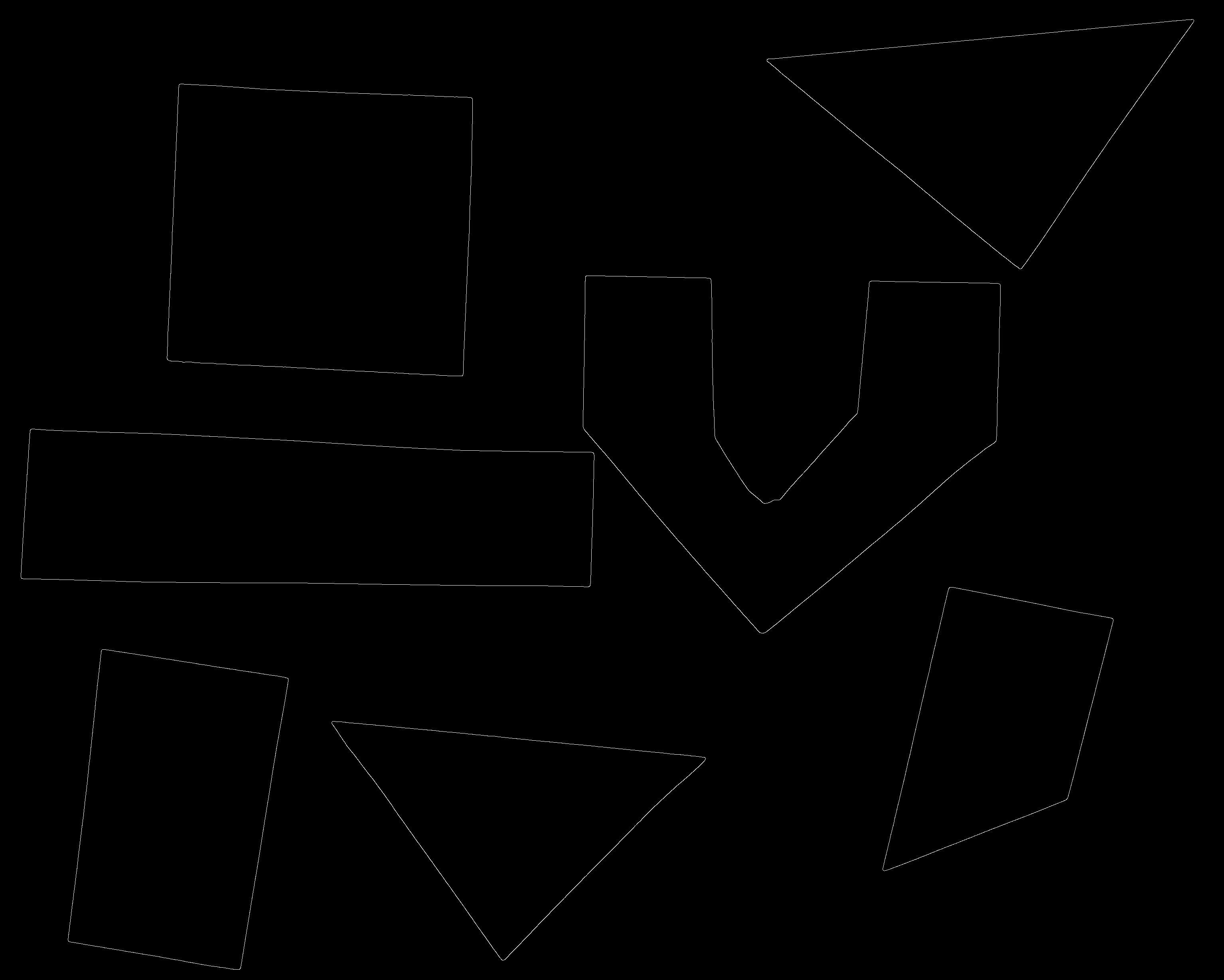
Note that the edge output shown in an skimage window may look significantly worse than the image would look if it were saved to a file due to resampling artefacts in the interactive image viewer. The image above is the edges of the junk image, saved in a PNG file. Here is how the same image looks when displayed in an skimage output window:
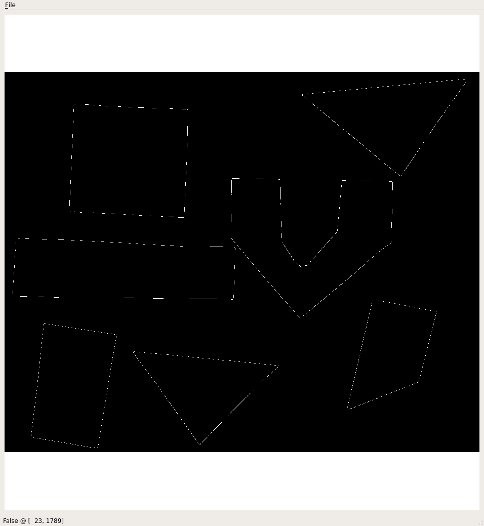
Interacting with the image viewer using viewer plugins
As we have seen, for a user of the skimage.feature.canny() edge detection function,
three important parameters to pass in are sigma, and the low and high threshold values used
in step four of the process. These values generally are determined empirically,
based on the contents of the image(s) to be processed.
Here is an image of some glass beads that we can use as input into a Canny edge detection program:
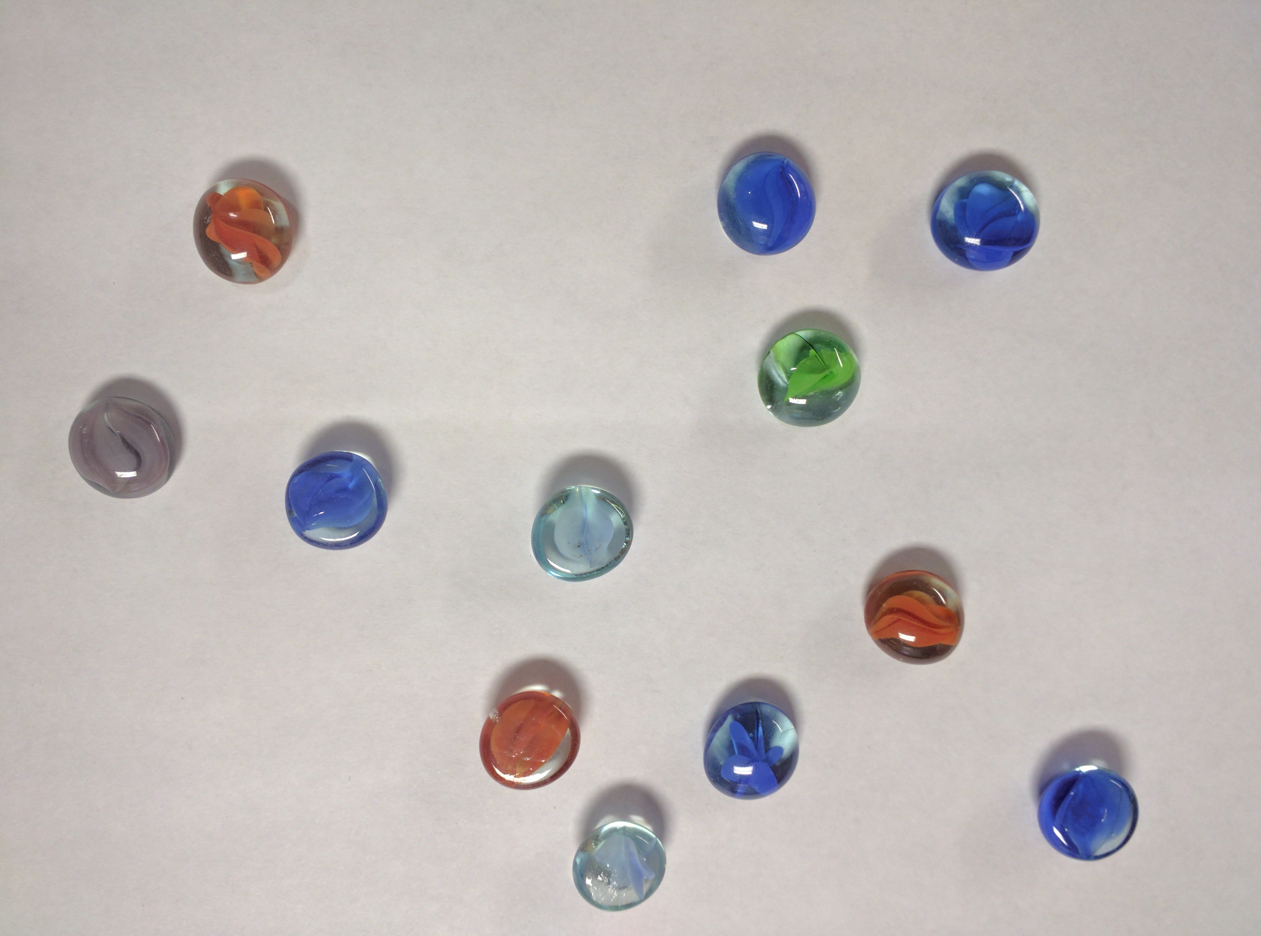
We could use the CannyEdge.py program above to find edges in this image. To find acceptable values for the thresholds, we would have to run the program over and over again, trying different threshold values and examining the resulting image, until we find a combination of parameters that works best for the image.
Or, we can write a Python program and create a viewer plugin that uses skimage sliders, that allow us to vary the function parameters while the program is running. In other words, we can write a program that presents us with a window like this:
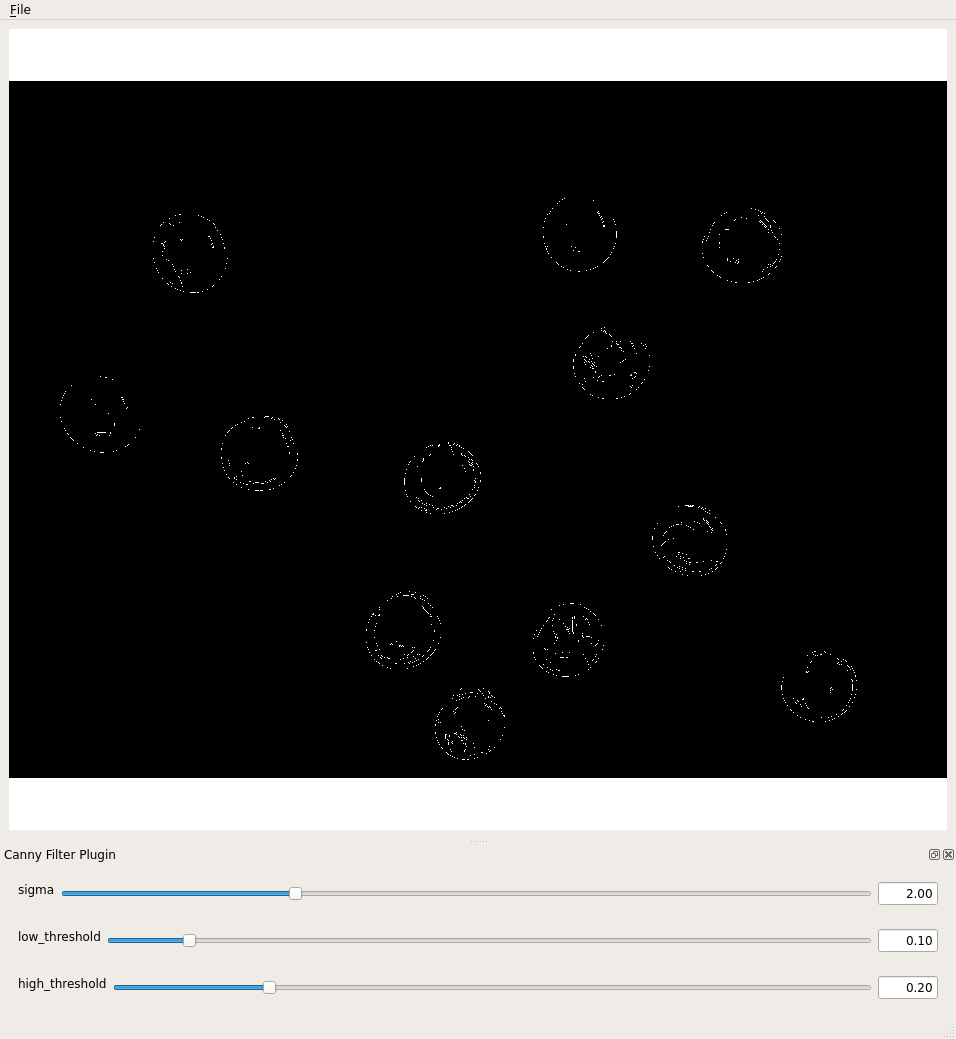
Then, when we run the program, we can use the sliders to vary the values of the sigma and threshold parameters until we are satisfied with the results. After we have determined suitable values, we can use the simpler program to utilize the parameters without bothering with the user interface and sliders.
Here is a Python program that shows how to apply Canny edge detection, and how to add sliders to the user interface. There are four parts to this program, making it a bit (but only a bit) more complicated than the programs we have looked at so far. The added complexity comes from setting up the sliders for the parameters that were previously read from the command line: In particular, we have added
- The
canny()filter function that returns an edge image, - The
cannyPluginplugin object, to which we add - The sliders for sigma, and low and high threshold values, and
- The main program, i.e., the code that is executed when the program runs.
We will look at the main program part first, and then return to writing the plugin. The first several lines of the main program are easily recognizable at this point: saving the command-line argument, reading the image in grayscale, and creating a window.
"""
 * Python script to demonstrate Canny edge detection
 * with sliders to adjust the thresholds.
 *
 * usage: python CannyTrack.py <filename>
"""
import skimage
import skimage.feature
import skimage.viewer
import sys


filename = sys.argv[1]
image = skimage.io.imread(fname=filename, as_gray=True)
viewer = skimage.viewer.ImageViewer(image)
The skimage.viewer.plugins.Plugin class is designed to manipulate images.
It takes an image_filter argument in the constructor that should be a function.
This function should produce a new image as an output, given an image as the first argument, which then will be automatically displayed in the image viewer.
# Create the plugin and give it a name
canny_plugin = skimage.viewer.plugins.Plugin(image_filter=skimage.feature.canny)
canny_plugin.name = "Canny Filter Plugin"
We want to interactively modify the parameters of the filter function interactively.
Skimage allows us to further enrich the plugin by adding widgets, like skimage.viewer.widgets.Slider, skimage.viewer.widgets.CheckBox, skimage.viewer.widgets.ComboBox.
Whenever a widget belonging to the plugin is updated, the filter function is called with the updated parameters.
This function is also called a callback function.
The following code adds sliders for sigma, low_threshold and high_thresholds.
# Add sliders for the parameters
canny_plugin += skimage.viewer.widgets.Slider(
    name="sigma", low=0.0, high=7.0, value=2.0
)
canny_plugin += skimage.viewer.widgets.Slider(
    name="low_threshold", low=0.0, high=1.0, value=0.1
)
canny_plugin += skimage.viewer.widgets.Slider(
    name="high_threshold", low=0.0, high=1.0, value=0.2
)
A slider is a widget that lets you choose a number by dragging a handle along a line.
On the left side of the line, we have the lowest value, on the right side the highest value that can be chosen.
The range of values in between is distributed equally along this line.
All three sliders are constructed in the same way:
The first argument is the name of the parameter that is tweaked by the slider.
With the arguments low, and high, we supply the limits for the range of numbers that is represented by the slider.
The value argument specifies the initial value of that parameter, so where the handle is located when the plugin is started.
Adding the slider to the plugin makes the values available as parameters to the filter_function.
How does the plugin know how to call the filter function with the parameters?
The filter function will be called with the slider parameters according to their names as keyword arguments. So it is very important to name the sliders appropriately.
Finally, we add the plugin the viewer and display the resulting user interface:
# add the plugin to the viewer and show the window
viewer += canny_plugin
viewer.show()
Here is the result of running the preceding program on the beads image, with a sigma value 1.0, low threshold value 0.1 and high threshold value 0.3. The image shows the edges in an output file.
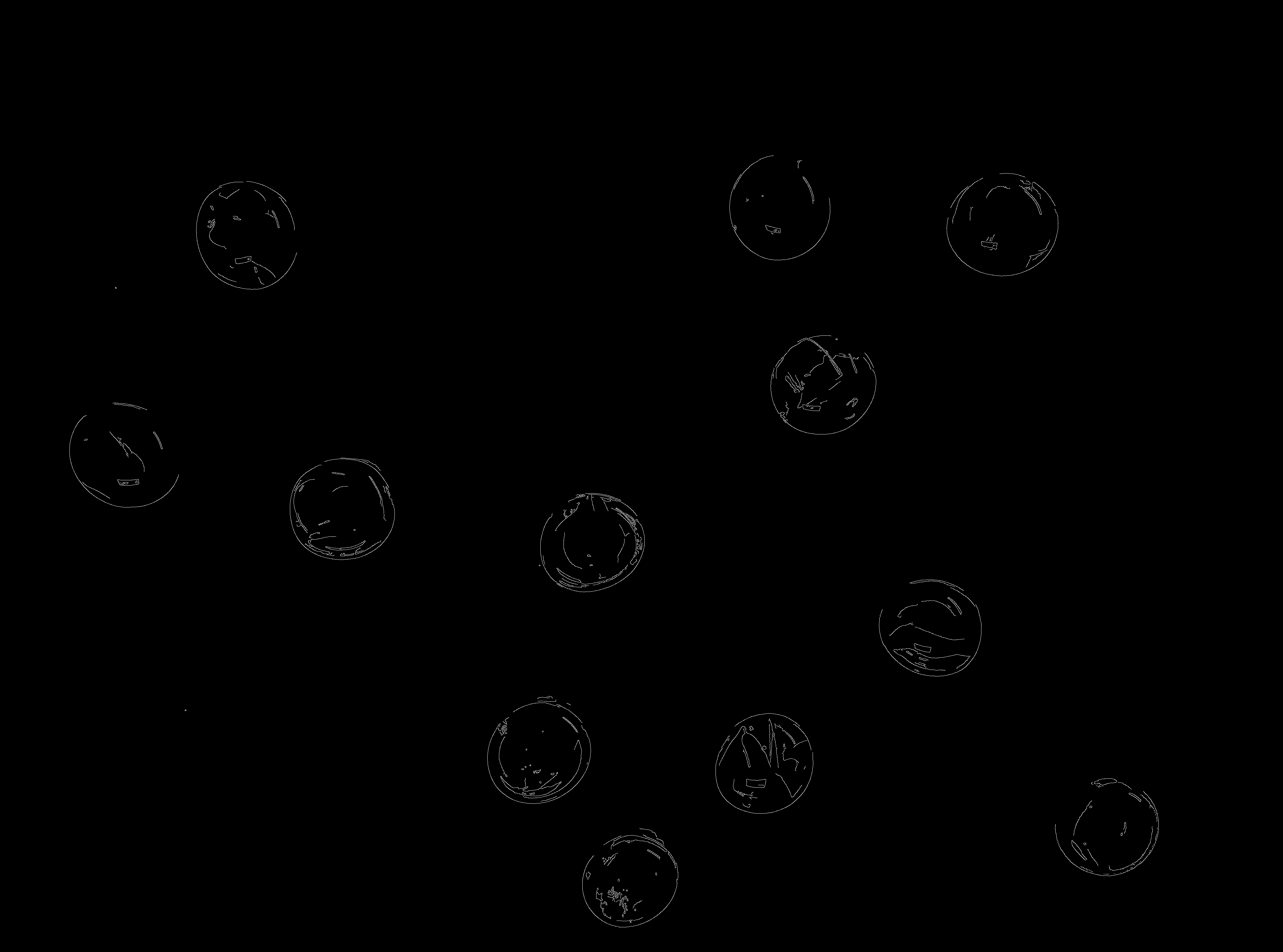
Applying Canny edge detection to another image (5 min)
Now, navigate to the Desktop/workshops/image-processing/08-edge-detection directory, and run the CannyTrack.py program on the image of colored shapes, junk.jpg. Use a sigma of 1.0 and adjust low and high threshold sliders to produce an edge image that looks like this:
What values for the low and high threshold values did you use to produce an image similar to the one above?
Solution
The colored shape edge image above was produced with a low threshold value of 0.05 and a high threshold value of 0.07. You may be able to achieve similar results with other threshold values.
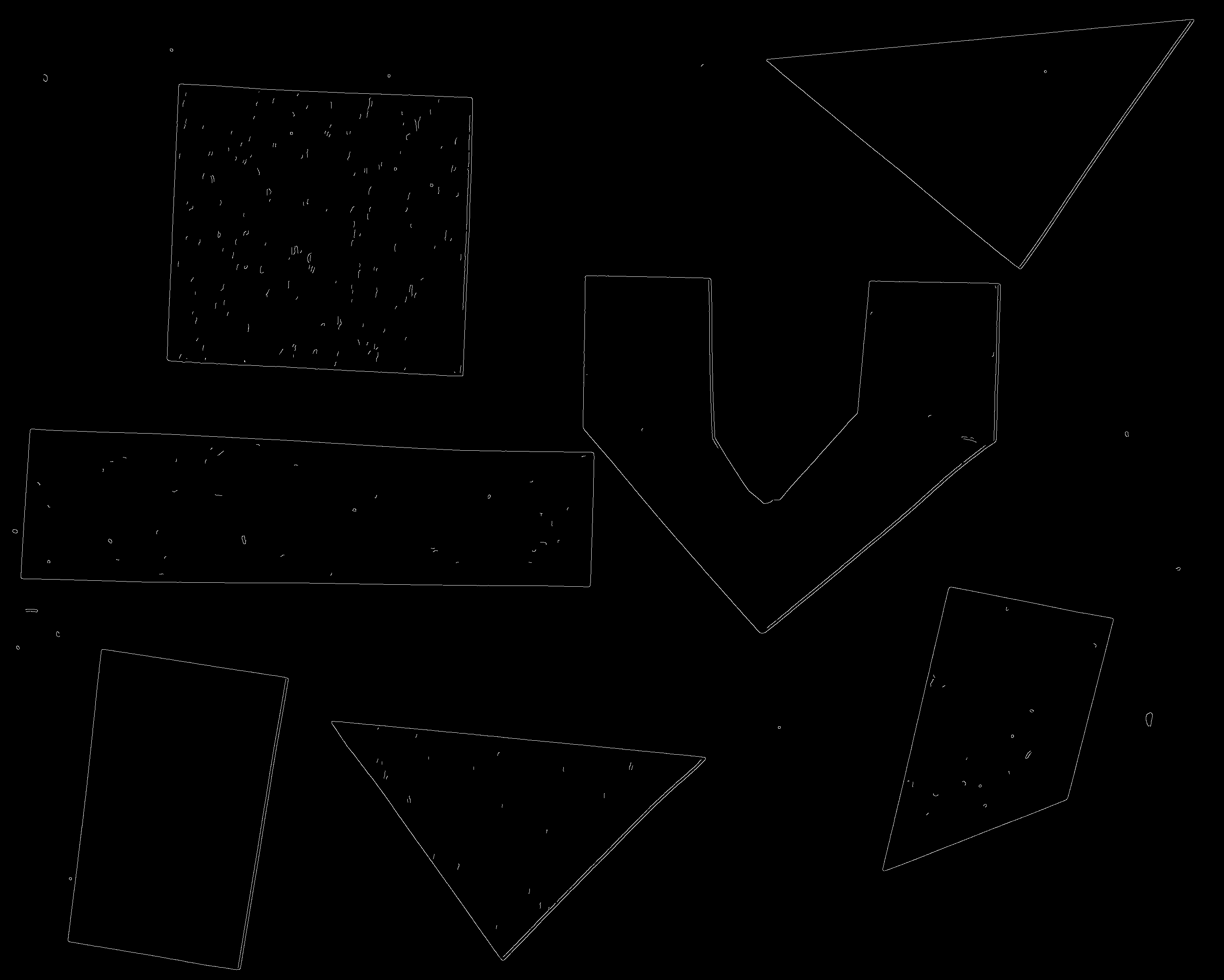
Using sliders for thresholding (30 min)
Now, let us apply what we know about creating sliders to another, similar situation. Consider this image of a collection of maize seedlings, and suppose we wish to use simple fixed-level thresholding to mask out everything that is not part of one of the plants.
To perform the thresholding, we could first create a histogram, then examine it, and select an appropriate threshold value. Here, however, let us create an application with a slider to set the threshold value. Create a program that reads in the image, displays it in a window with a slider, and allows the slider value to vary the threshold value used. You will find the image in the Desktop/workshops/image-processing/08-edge-detection directory, under the name maize-roots.jpg.
Solution
Here is a program that uses a slider to vary the threshold value used in a simple, fixed-level thresholding process.
"""
 * Python program to use a slider to control fixed-level
 * thresholding value.
 *
 * usage: python interactive_thresholding.py <filename>
"""

import skimage
import skimage.viewer
import sys

filename = sys.argv[1]


def filter_function(image, sigma, threshold):
    masked = image.copy()
    masked[skimage.filters.gaussian(image, sigma=sigma) <= threshold] = 0
    return masked


smooth_threshold_plugin = skimage.viewer.plugins.Plugin(
    image_filter=filter_function
)

smooth_threshold_plugin.name = "Smooth and Threshold Plugin"

smooth_threshold_plugin += skimage.viewer.widgets.Slider(
    "sigma", low=0.0, high=7.0, value=1.0
)
smooth_threshold_plugin += skimage.viewer.widgets.Slider(
    "threshold", low=0.0, high=1.0, value=0.5
)

image = skimage.io.imread(fname=filename, as_gray=True)

viewer = skimage.viewer.ImageViewer(image=image)
viewer += smooth_threshold_plugin
viewer.show()
Here is the output of the program, blurring with a sigma of 1.5 and a threshold value of 0.45:
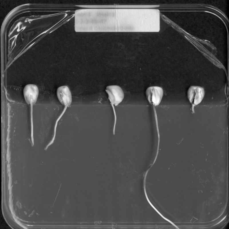
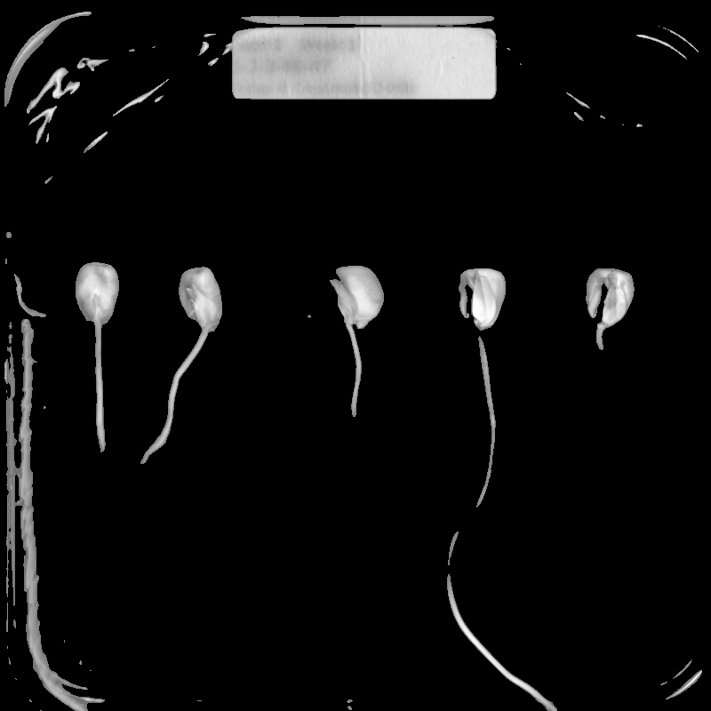
Keep this plugin technique in your image processing “toolbox.” You can use sliders (or other interactive elements, see the skimage documentation) to vary other kinds of parameters, such as sigma for blurring, binary thresholding values, and so on. A few minutes developing a program to tweak parameters like this can save you the hassle of repeatedly running a program from the command line with different parameter values. Furthermore, skimage already comes with a few viewer plugins that you can check out in the documentation.
Other edge detection functions
As with blurring, there are other options for finding edges in skimage. These
include skimage.filters.sobel(), which you will recognize as part of the Canny
method. Another choice is skimage.filters.laplace().
Key Points
The
skimage.viewer.ImageVieweris extended using askimage.viewer.plugins.Plugin.We supply a filter function callback when creating a Plugin.
Parameters of the callback function are manipulated interactively by creating sliders with the
skimage.viewer.widgets.slider()function and adding them to the plugin.
Connected Component Analysis
Overview
Teaching: ?? min
Exercises: ?? minQuestions
How to extract separate objects from an image and describe these objects quantitatively.
Objectives
Understand the term object in the context of images.
Learn about pixel connectivity.
Learn how Connected Component Analysis (CCA) works.
Use CCA to produce an image that highlights every object in a different color.
Characterize each object with numbers that describe its appearance.
Objects
In the thresholding episode we have covered dividing an image in foreground and background pixels. In the junk example image, we considered the colored shapes as foreground objects on a white background.
In thresholding we went from the original image to this version:
Here, we created a mask that only highlights the parts of the image that we find interesting, the objects.
All objects have pixel value of True while the background pixels are False.
By looking at the mask image, one can count the objects that are present in the image (7). But how did we actually do that, how did we decide which lump of pixels constitutes a single object?
Pixel Neighborhoods
In order to decide which pixels belong to the same object, one can exploit their neighbourhood: pixels that are directly next to each other and belong to the foreground class can be considered to belong to the same object.
Let’s consider the following mask “image” with 8 rows, and 8 columns.
Note that for brevity, 0 is used to represent False (background) and 1 to represent True (foreground).
0 0 0 0 0 0 0 0
0 1 1 0 0 0 0 0
0 1 1 0 0 0 0 0
0 0 0 1 1 1 0 0
0 0 0 1 1 1 1 0
0 0 0 0 0 0 0 0
The pixels are organized in a rectangular grid.
In order to understand pixel neighborhoods we will introduce the concept of “jumps” between pixels.
The jumps follow two rules:
First rule is that one jump is only allowed along the column, or the row.
Diagonal jumps are not allowed.
So, from a center pixel, denoted with o, only the pixels indicated with an x are reachable:
- x -
x o x
- x -
The pixels on the diagonal (from o) are not reachable with a single jump, which is denoted by the -.
The pixels reachable with a single jump form the 1-jump neighborhood.
The second rule states that in a sequence of jumps, one may only jump in row and column direction once -> they have to be orthogonal.
An example of a sequence of orthogonal jumps is shown below.
Starting from o the first jump goes along the row to the right.
The second jump then goes along the column direction up.
After this the sequence cannot be continued as a jump has been made in row and column direction.
- - 2
- o 1
- - -
All pixels reachable with one, or two jumps form the 2-jump neighborhood.
The grid below illustrates the pixels reachable from the center pixel o with a single jump, highlighted with a 1, and the pixels reachable with 2 jumps with a 2.
2 1 2
1 o 1
2 1 2
We want to revisiting our example image mask from above and apply the two different neighborhood rules.
With a single jump connectivity for each pixel, we get two resulting objects, highlighted in the image with 1’s and 2’s.
0 0 0 0 0 0 0 0
0 1 1 0 0 0 0 0
0 1 1 0 0 0 0 0
0 0 0 2 2 2 0 0
0 0 0 2 2 2 2 0
0 0 0 0 0 0 0 0
In the 1-jump version, only pixels that neighbors in rows or columns, are considered connected. With two jumps, however, we only get a single objects, as pixels are also considered connected along the diagonals.
0 0 0 0 0 0 0 0
0 1 1 0 0 0 0 0
0 1 1 0 0 0 0 0
0 0 0 1 1 1 0 0
0 0 0 1 1 1 1 0
0 0 0 0 0 0 0 0
Exercise: Object counting
How many objects with 1 orthogonal jump, how many with 2 orthogonal jumps?
0 0 0 0 0 0 0 0
0 1 0 0 0 1 1 0
0 0 1 0 0 0 0 0
0 1 0 1 1 1 0 0
0 1 0 1 1 0 0 0
0 0 0 0 0 0 0 0
1 jump
a) 1 b) 5 c) 2
Solution
b) 5
2 jumps
a) 2 b) 3 c) 5
Solution
a) 2
Jumps and neighborhoods
We have just introduced how you can reach different neighboring pixels by performing one or more orthogonal jumps. There is also a different way of referring to these pixels: the 4- and 8-neighborhood. With a single jump you can reach four pixels from a given starting pixel. Hence, the one jump neighborhood corresponds to the 4-neighborhood. When two orthogonal jumps are allowed, eight pixels can be reached, so this corresponds to the 8-neighborhood.
Connected Component Analysis
In order to find the objects in an image, we want to employ an operation that is called Connected Component Analysis (CCA).
This operation takes a binary image as an input.
Usually, the False value in this image is associated with background pixels, and the True value indicates foreground, or object pixels.
Such an image can be e.g. produced with thresholding.
Given a thresholded image, CCA produces a new labeled image with integer pixel values.
Pixels with the same value, belong to the same object.
We use the thresholding script as a starting point to write a program, that prints the number of objects in an image.
"""
 * Python script count objects in an image
 *
 * usage: python CCA.py <filename> <sigma> <threshold>
"""
import sys
import numpy as np
import skimage.color
import skimage.filters
import skimage.io
import skimage.viewer
import skimage.measure
import skimage.color

# get filename, sigma, and threshold value from command line
filename = sys.argv[1]
sigma = float(sys.argv[2])
t = float(sys.argv[3])

# read and display the original image
image = skimage.io.imread(fname=filename, as_gray=True)
viewer = skimage.viewer.ImageViewer(image)
viewer.show()

# blur and grayscale before thresholding
blur = skimage.filters.gaussian(image, sigma=sigma)

# perform inverse binary thresholding
mask = blur < t

# display the result
viewer = skimage.viewer.ImageViewer(mask)
viewer.show()

# Perform CCA on the mask
labeled_image = skimage.measure.label(mask, connectivity=2, return_num=True)

viewer = skimage.viewer.ImageViewer(labeled_image)
viewer.show()
Let’s examine the changes to the original thresholding script.
There is an additional import: skimage.measure.
We import skimage.measure in order to use the skimage.measure.label function that performs CCA.
After the imports, the parameters for sigma and the threshold are read from the command line.
The original image is displayed first, then blurring and thresholding is performed.
The resulting binary image is also displayed in an interactive viewer.
The new code follows the comment Perform CCA on the mask.
The skimage function to perform CCA is skimage.measure.label.
It has one positional argument, where we supply mask, the binary image to work on.
With an optional argument we, specify the connectivity in units of orthogonal jumps.
By setting connectivity=2 we will consider a particular pixel connected to a second one, if the second one is reachable with two orthogonal jumps from the first pixel.
The function returns an image in which each object is represented with a unique pixel value.
We assign this image to the variable labeled_image.
Calling the script with the junk.jpg image and sigma=2.0 and threshold=0.9 yields an all black image.
Note: this behavior might change in future versions, or not occur with a different image viewer.
What went wrong?
When we hover with the mouse over this black image, the underlying pixel values are shown as numbers in the lower left corner.
We can see that in some positions they are not 0, but still this image is black.
Let’s find out more by examining label_image.
Properties that might be interesting in this context are dtype, the minimum and maximum value.
We can do so by adding the following lines:
print("dtype:", label_image.dtype)
print("min:", numpy.min(label_image))
print("max:", numpy.max(label_image))
Examining the output can give us a clue:
dtype: int64
min: 0
max: 11
The dtype of label_image is int64.
This means that values in this image range from -2 ** 63 to 2 ** 63 - 1.
Those are really big numbers.
From this available space we only use the range from 0 to 11.
When showing this image in the viewer, it squeezes the complete range into 256 gray values.
The range of our numbers does not produce any visible change.
The skimage library has tools to cope with this a situation.
In the skimage.color module has a function label2rgb() that will do the conversion.
We have already used the skimage.color module to convert color images to gray scale images.
skimage.color.label2rgb() will create a new color image.
All objects are colored according to a list of colors that can be customized.
In order to see our objects, we can add the following code to our program:
# convert the label image to color image
colored_label_image = skimage.color.label2rgb(labeled_image, bg_label=0)

# show the created image in the viewer
viewer = skimage.viewer.ImageViewer(colored_label_image)
viewer.show()
How many objects are in that image (15 min)
Now, it is your turn to practice. Using the original
junk.pngimage, copy theCCA.pyscript to a new fileCCA-count.py. Modify this script to print out the number of found objects in the end.
What number of objects would you expect to get? How does changing the
sigmaandthresholdvalues influence the result?Solution
All pixels that belong to a single object are assigned the same integer value. The algorithm produces consecutive numbers. That means the first object gets the value
1, the second object the value2and so on. This means that, by finding the object with the maximum value, we know how many objects there are in the image. Using thenumpy.maxfunction will give us the maximum value in the imageAdding the following code at the end of the
CCA-count.pyprogram will print out the number of objectsnum_objects = numpy.max(labeled_image) print("Found", num_objects, "objects in the image.")Invoking the program with
sigma=2.0, andthreshold=0.9will printFound 11 objects in the image.Lowering the threshold will result in fewer objects. The higher the threshold is set, the more objects are found. More and more background noise gets picked up as objects.
Larger sigmas produce binary masks with less noise and hence a smaller number of objects. Setting sigma too high bears the danger of merging objects.
Morphometrics - Describe object features with numbers
Plot a histogram of the object area distribution (15 min)
In the previous exercise we wrote the
CCA-count.pyprogram and explored how the object count changed with the parameters. We had a hard time making the script print out the right number of objects. In order to get closer to a solution to this problem, we want to look at the distribution of the object areas. Calculate the object properties usingskimage.measure.regionpropsand generate a histogram.Make a copy of the
CCA.pyscript and modify it to also produce a plot of the histogram of the object area.What does the histogram tell you about the objects?
Hint: Try to generate a list of object areas first.
Solution
# add the import for pyplot
from matplotlib import pyplot as plt

# compute object features and extrac object areas
object_features = skimage.measure.regionprops(labeled_image)
object_areas = [objf["area"] for objf in object_features]
plt.hist(object_areas)
plt.show()
Filter objects by area (15 min)
Our
CCA-count.pyprogram has an apparent problem: it is hard to find a combination that produces the right output number. In some cases the problem arose that some background noise got picked up as an object. With other parameter settings some of the foreground objects got broken up or disappeared completely.
Modify the program in order to only count large objects.
Solution
Now make this change visual: Modify the label image such that objects below a certain area are set to the background label (0).
Solution
# iterate over object_ids and modify the `labeled_image` in-place
for object_id, objf in enumerate(object_features, start=1):
    if objf["area"] < 10000:
        labeled_image[labeled_image == object_id] = 0
Lastly print out the count for the large objects
Solution
# generate a list of objects above a certain area
filtered_list = []
for objf in object_features:
    if objf["area"] > 10000:
        filtered_list.append(objf["area"])

print("Found", len(filtered_list), "objects!")
The script, if working properly, will produce the following output:
Fount 7 objects!
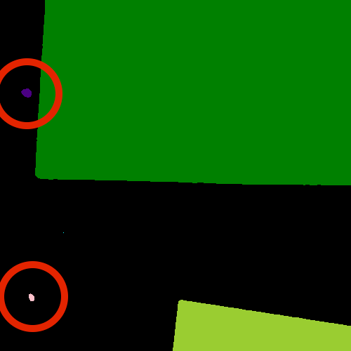
Key Points
skimage.measure.labelis used to generate objects.We use
skimage.measure.regionpropsto measure properties of labelled objects.Color objects according to feature values.
Challenges
Overview
Teaching: 30 min
Exercises: 0 minQuestions
What are the questions?
Objectives
What are the objectives?
In this episode, we will provide two different challenges for you to attempt, based on the skills you have acquired so far. One of the challenges will be related to the shape of objects in images (morphometrics), while the other will be related to colors of objects in images (colorimetrics). We will not provide solution code for either of the challenges, but your instructors should be able to give you some gentle hints if you need them.
Morphometrics: Bacteria Colony Counting
As mentioned in the workshop introduction, your morphometric challenge is to determine how many bacteria colonies are in each of these images. These images can be found in the Desktop/workshops/image-processing/10-challenges/morphometric directory.

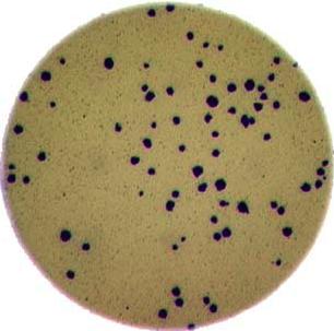
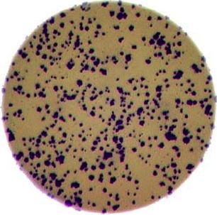
Write a Python program that uses skimage to count the number of bacteria colonies in each image, and for each, produce a new image that highlights the colonies. The image should look similar than this one:
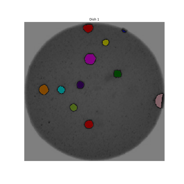
Additionally, print out the number of colonies for each image.

Colorimetrics: titration color analysis
The video showing the titration process first mentioned in the workshop introduction episode can be found in the Desktop/workshops/image-processing/10-challenges/colorimetric directory. Write a Python program that uses skimage to analyze the video on a frame-by-frame basis. Your program should do the following:
-
Sample a kernel from the same location on each frame, and determine the average red, green, and blue channel value.
-
Display a graph plotting the average color channel values as a function of the frame number, similar to this image:
-
Save the graph as an image named titration.png.
-
Output a CSV file named titration.csv, with each line containing the frame number, average red value, average green value, and average blue value
Key Points
What are the key points?