Thresholding
Overview
Teaching: 30 min
Exercises: 65 minQuestions
How can we use thresholding to produce a binary image?
Objectives
Explain what thresholding is and how it can be used.
Use histograms to determine appropriate threshold values to use for the thresholding process.
Apply simple, fixed-level binary thresholding to an image.
Explain the difference between using the operator
>or the operator<to threshold an image represented by a numpy array.Describe the shape of a binary image produced by thresholding via
>or<.Explain when Otsu’s method of adaptive thresholding is appropriate.
Apply adaptive thresholding to an image using Otsu’s method.
Use the
np.nonzero()function to count the number of non-zero pixels in an image.
In this episode, we will learn how to use skimage functions to apply thresholding to an image. Thresholding is a type of image segmentation, where we change the pixels of an image to make the image easier to analyze. In thresholding, we convert an image from color or grayscale into a binary image, i.e., one that is simply black and white. Most frequently, we use thresholding as a way to select areas of interest of an image, while ignoring the parts we are not concerned with. We have already done some simple thresholding, in the “Manipulating pixels” section of the Skimage Images episode. In that case, we used a simple NumPy array manipulation to separate the pixels belonging to the root system of a plant from the black background. In this episode, we will learn how to use skimage functions to perform thresholding. Then, we will use the masks returned by these functions to select the parts of an image we are interested in.
Simple thresholding
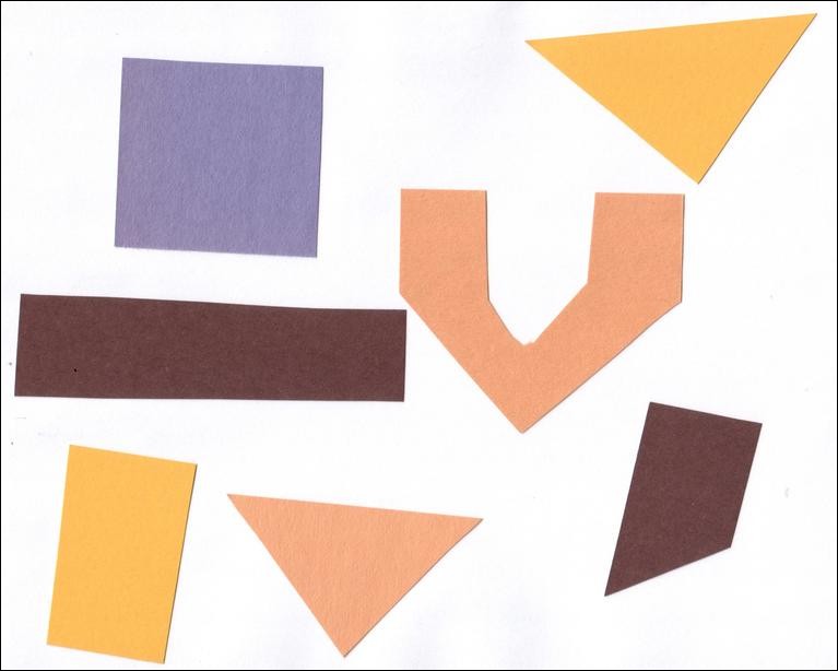
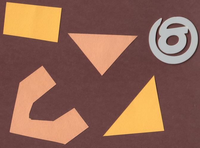
Consider this image, with a series of crudely cut shapes set against a white background. The black outline around the image is not part of the image.
Now suppose we want to select only the shapes from the image. In other words,
we want to leave the pixels belonging to the shapes “on,” while turning the
rest of the pixels “off,” by setting their color channel values to zeros. The
skimage library has several different methods of thresholding. We will start
with the simplest version, which involves an important step of human
input. Specifically, in this simple, fixed-level thresholding, we have to
provide a threshold value, t.
The process works like this. First, we will load the original image, convert
it to grayscale, and blur it with one of the methods from the
Blurring episode. Then, we will use the
> operator to apply the threshold t, a number in the closed range [0.0, 1.0].
Pixels with color values on one
side of t will be turned “on,” while pixels with color values on the other side
will be turned “off.” In order to use this function, we have to determine a good
value for t. How might we do that? Well, one way is to look at a grayscale
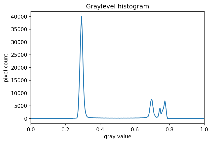
histogram of the image. Here is the histogram produced by the
GrayscaleHistogram.py program from the
Creating Histograms episode, if we
run it on the colored shapes image shown above.
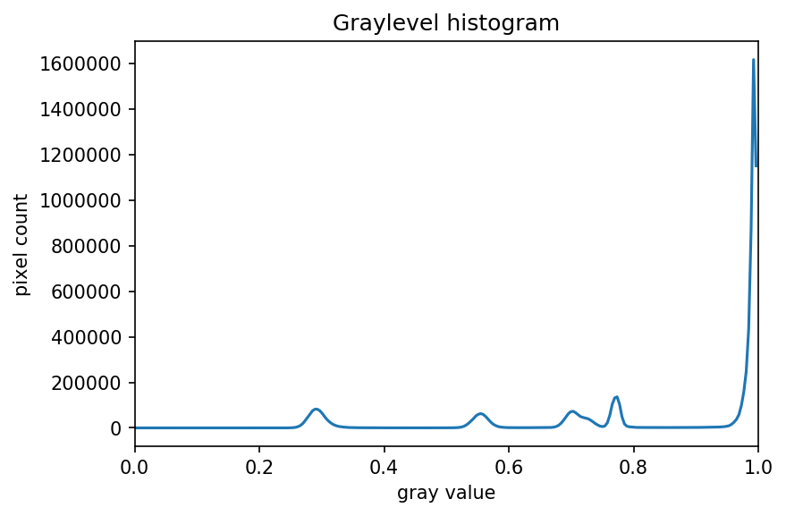
Since the image has a white background, most of the pixels in the image are
white. This corresponds nicely to what we see in the histogram: there is a
spike near the value of 1.0. If we want to select the shapes and not the
background, we want to turn off the white background pixels, while leaving the
pixels for the shapes turned on. So, we should choose a value of t somewhere
before the large peak and turn pixels above that value “off”.
Here are the first few lines of a Python program to apply simple thresholding to the image, to accomplish this task.
"""
 * Python script to demonstrate simple thresholding.
 *
 * usage: python Threshold.py <filename> <sigma> <threshold>
"""
import sys
import numpy as np
import skimage.color
import skimage.filters
import skimage.io
import skimage.viewer

# get filename, sigma, and threshold value from command line
filename = sys.argv[1]
sigma = float(sys.argv[2])
t = float(sys.argv[3])

# read and display the original image
image = skimage.io.imread(fname=filename)
viewer = skimage.viewer.ImageViewer(image)
viewer.show()
This program takes three command-line arguments: the filename of the image to
manipulate, the sigma of the Gaussian used during the blurring step (which, if you recall
from the Blurring episode, must be a float),
and finally, the threshold value t, which should be a float in the closed
range [0.0, 1.0]. The program takes the command-line values and stores them in
variables named filename, sigma, and t, respectively.
Next, the program reads the original image based on the filename value, and
displays it.
Now is where the main work of the program takes place.
# blur and grayscale before thresholding
blur = skimage.color.rgb2gray(image)
blur = skimage.filters.gaussian(blur, sigma=k)
First, we convert the
image to grayscale and then blur it, using the skimage.filter.gaussian() function we
learned about in the Blurring episode.
We convert the input image to grayscale for easier thresholding.
The fixed-level thresholding is performed using numpy comparison operators.
# perform inverse binary thresholding
mask = blur < t_rescaled
Here, we want to turn “on” all pixels which have values smaller than the threshold,
so we use the less operator < to compare the blurred image blur to the threshold t.
The operator returns a binary image, that we capture in the variable mask.
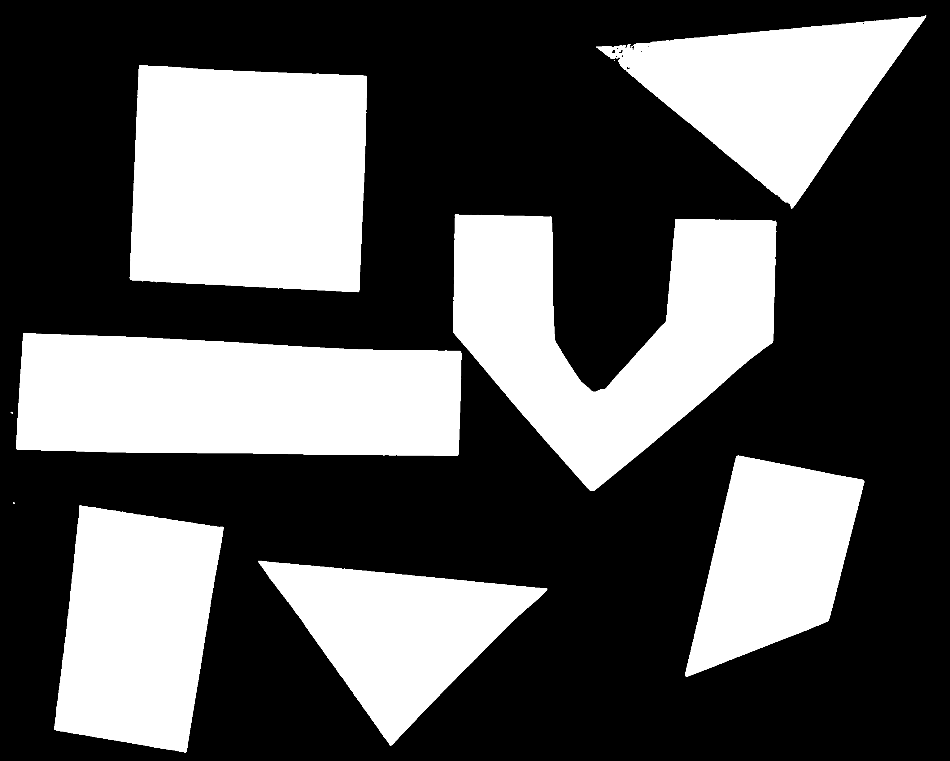
It has only one channel, and each of its values is either 0 or 1. Here is a
visualization of the binary image created by the thresholding operation.
The program used parameters of sigma = 2 and t = 0.8 to produce this image. You can
see that the areas where the shapes were in the original area are now white,
while the rest of the mask image is black.
We can now apply the mask to the original colored image as we have learned in the Drawing and Bitwise Operations episode.
# use the mask to select the "interesting" part of the image
sel = np.zeros_like(image)
sel[mask] = image[mask]

# display the result
viewer = skimage.viewer.ImageViewer(sel)
viewer.view()
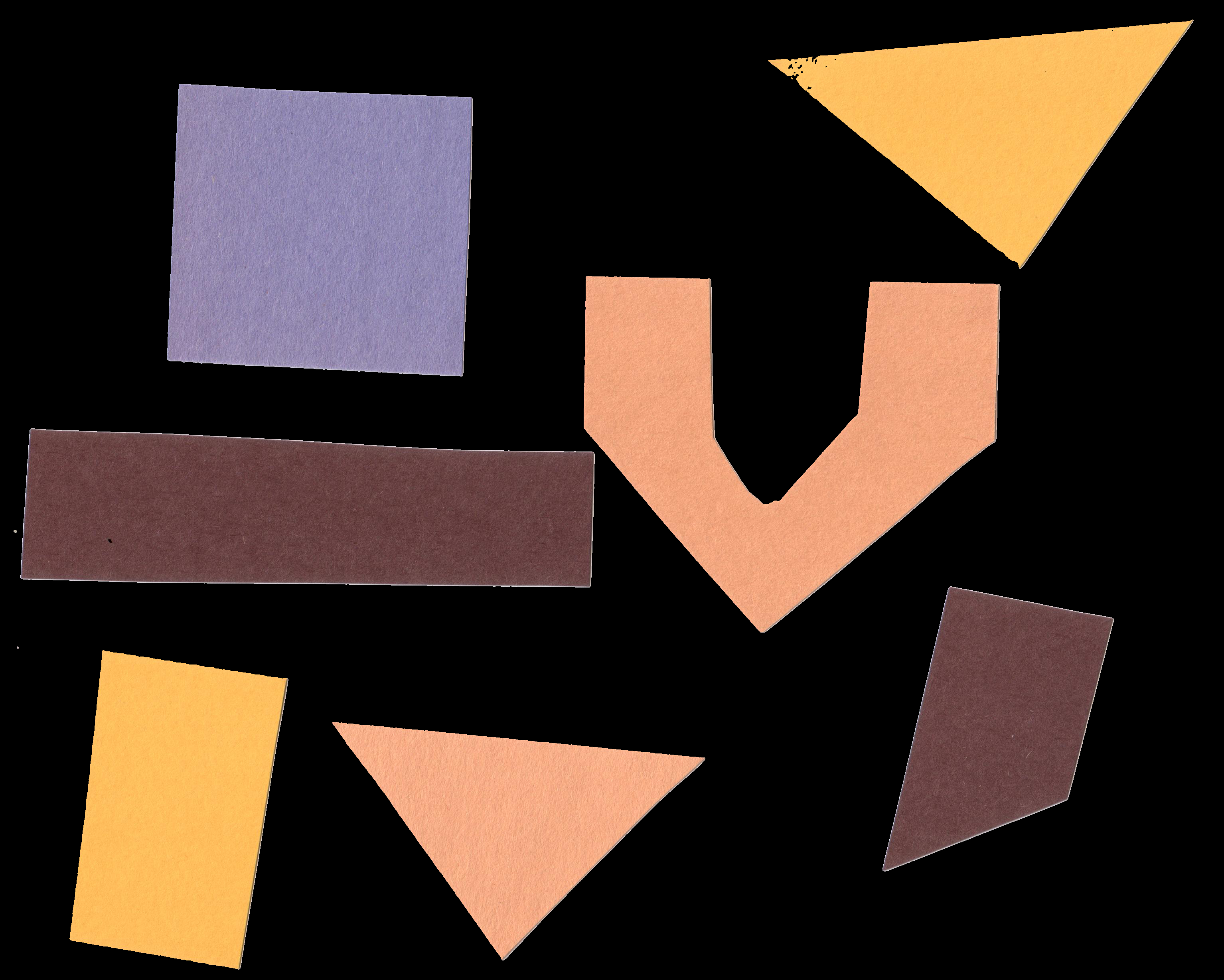
What we are left with is only the colored shapes from the original, as shown in this image:
More practice with simple thresholding (15 min)
Now, it is your turn to practice. Suppose we want to use simple thresholding to select only the colored shapes from this image:
First, use the GrayscaleHistogram.py program in the Desktop/workshops/image-processing/05-creating-histograms directory to examine the grayscale histogram of the more-junk.jpg image, which you will find in the Desktop/workshops/image-processing/07-thresholding directory. Via the histogram, what do you think would be a good value for the threshold value,
t?Solution
Here is the histogram for the more-junk.jpg image.
We can see a large spike around 0.3, and a smaller spike around 0.7. The spike near 0.3 represents the darker background, so it seems like a
tvalue close to 0.5 would be a good choice.Now, modify the ThresholdPractice.py program in the Desktop/workshops/image-processing/07-thresholding directory to turn the pixels above the
tvalue on and turn the pixels below thetvalue off. To do this, change the comparison operator less<to greater>. Then execute the program on the more-junk.jpg image, using a reasonable value for k and thetvalue you obtained from the histogram. If everything works as it should, your output should show only the colored shapes on a pure black background.Solution
Here is the modified ThresholdPractice.py program.
"""
 * Python script to practice simple thresholding.
 *
 * usage: python ThresholdPractice.py <filename> <sigma> <threshold>
"""
import sys
import numpy as np
import skimage.color
import skimage.fiters
import skimage.io
import skimage.viewer

# get filename, sigma, and threshold value from command line
filename = sys.argv[1]
sigma = float(sys.argv[2])
t = float(sys.argv[3])

# read and display the original image
image = skimage.io.imread(fname=filename)
viewer = skimage.viewer.ImageViewer(image)
viewer.show()

# blur and grayscale before thresholding
blur = skimage.color.rgb2gray(image)
blur = skimage.filters.gaussian(blur, sigma=sigma)

# perform binary thresholding
# MODIFY CODE HERE!
mask = blur > t

# display the mask image
viewer = skimage.viewer.ImageViewer(mask)
viewer.show()

# use the mask to select the "interesting" part of the image
sel = np.zeros_like(image)
sel[mask] = image[mask]

# display the result
viewer = skimage.viewer.ImageViewer(sel)
viewer.show()
Using a Gaussian with sigma = 2 and threshold t = 0.5, we obtain this mask:
And applying the mask results in this selection of shapes:


Adaptive thresholding
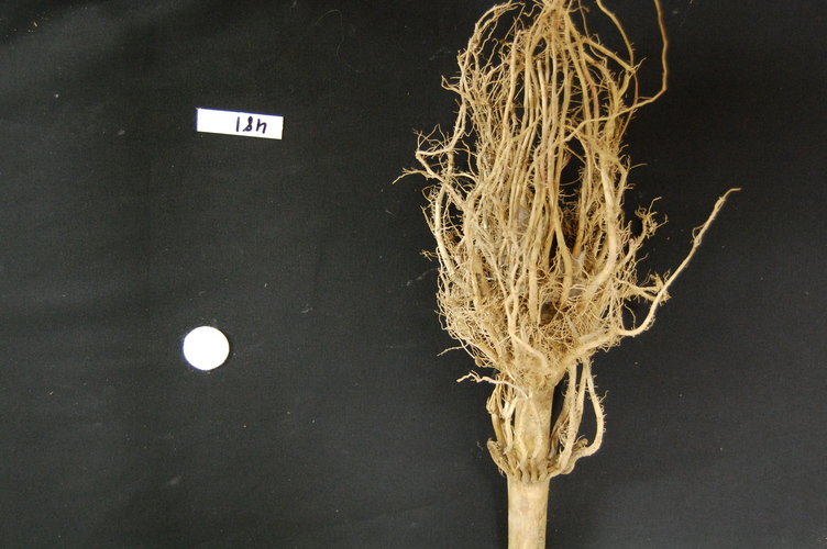
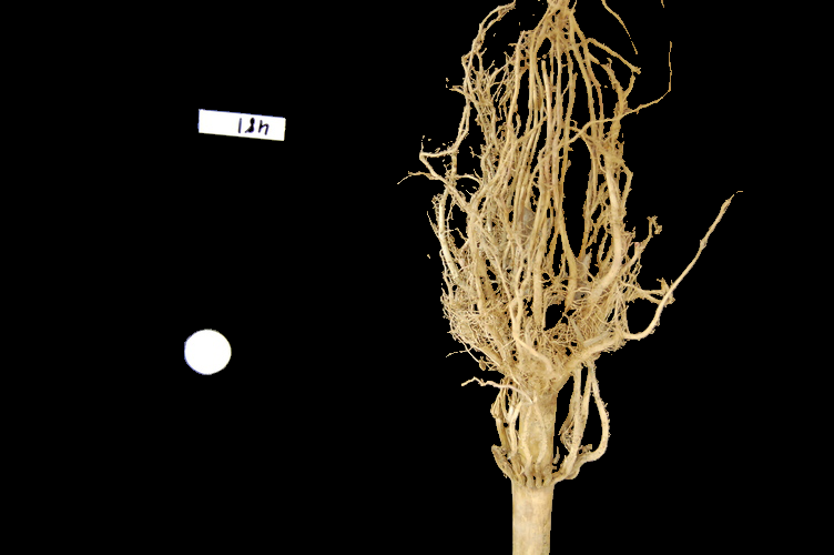
There are also skimage methods to perform adaptive thresholding. The chief advantage of adaptive thresholding is that the value of the threshold, t, is determined automatically for us. One such method, Otsu’s method, is particularly useful for situations where the grayscale histogram of an image has two peaks. Consider this maize root system image, which we have seen before in the Skimage Images episode.
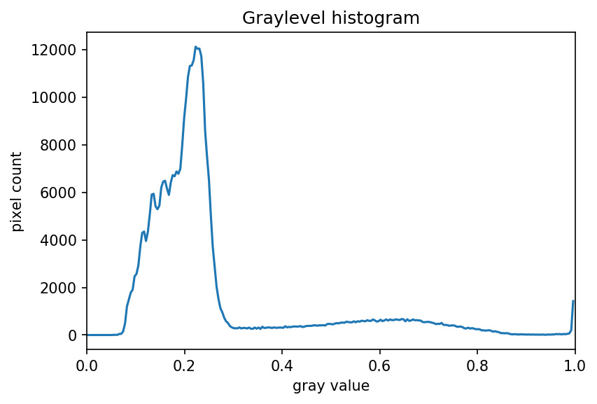
Now, look at the grayscale histogram of this image, as produced by our GrayscaleHistogram.py program from the Creating Histograms episode.

The histogram has a significant peak around 0.2, and a second, albeit smaller peak very near 1.0. Thus, this image is a good candidate for thresholding with Otsu’s method. The mathematical details of how this work are complicated (see the skimage documentation if you are interested), but the outcome is that Otsu’s method finds a threshold value between the two peaks of a grayscale histogram.
The skimage.filters.threshold_otsu() function can be used to determine
the adaptive threshold via Otsu’s method. Then numpy comparison operators can be
used to apply it as before.
Here is a Python program illustrating how to perform thresholding with Otsu’s
method using the skimage.filters.threshold_otsu function. We start by reading and displaying
the target image.
"""
 * Python script to demonstrate adaptive thresholding using Otsu's method.
 *
 * usage: python AdaptiveThreshold.py <filename> <sigma>
"""
import sys
import numpy as np
import skimage.color
import skimage.filters
import skimage.io
import skimage.viewer

# get filename and sigma value from command line
filename = sys.argv[1]
sigma = float(sys.argv[2])

# read and display the original image
image = skimage.io.imread(fname=filename)
viewer = skimage.viewer.ImageViewer(image)
viewer.show()
The program begins with the now-familiar imports and command line parameters.
Here we only have to get the filename and the sigma of the Gaussian kernel from the command
line, since Otsu’s method will automatically determine the thresholding value
t. Then, the original image is read and displayed.
Next, a blurred grayscale image is created.
# blur and grayscale before thresholding
blur = skimage.color.rgb2gray(image)
blur = skimage.filters.gaussian(image, sigma=sigma)
We determine the threshold via the skimage.filters.threshold_otsu() function:
# perform adaptive thresholding
t = skimage.filters.threshold_otsu(blur)
mask = blur > t
The function skimage.filters.threshold_otsu() uses Otsu’s method to automatically
determine the threshold value based on its inputs grayscale histogram and returns it.
Then, we use the comparison operator > for binary thesholding. As we have seen before,
pixels above the threshold value will be turned on, those below the threshold will be turned off.
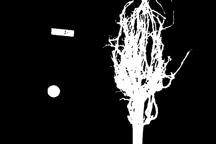
For this root image, and a Gaussian blur with a sigma of 1.0, the computed threshold value is 0.42, and the resulting mask is:
Next, we display the mask and use it to select the foreground
viewer = skimage.viewer.ImageViewer(mask)
viewer.show()

# use the mask to select the "interesting" part of the image
sel = np.zeros_like(image)
sel[mask] = image[mask]

# display the result
viewer = skimage.viewer.ImageViewer(sel)
viewer.show()
Here is the result:
Application: measuring root mass
Let us now turn to an application where we can apply thresholding and other techniques we have learned to this point. Consider these four maize root system images.

Now suppose we are interested in the amount of plant material in each image, and in particular how that amount changes from image to image. Perhaps the images represent the growth of the plant over time, or perhaps the images show four different maize varieties at the same phase of their growth. In any case, the question we would like to answer is, “how much root mass is in each image?” We will construct a Python program to measure this value for a single image, and then create a Bash script to execute the program on each trial image in turn.
Our strategy will be this:
- Read the image, converting it to grayscale as it is read. For this application we do not need the color image.
- Blur the image.
- Use Otsu’s method of thresholding to create a binary image, where the pixels that were part of the maize plant are white, and everything else is black.
- Save the binary image so it can be examined later.
- Count the white pixels in the binary image, and divide by the number of pixels in the image. This ratio will be a measure of the root mass of the plant in the image.
- Output the name of the image processed and the root mass ratio.
Here is a Python program to implement this root-mass-measuring strategy. Almost all of the code should be familiar, and in fact, it may seem simpler than the code we have worked on thus far, because we are not displaying any of the images with this program. Our program here is intended to run and produce its numeric result – a measure of the root mass in the image – without human intervention.
"""
 * Python program to determine root mass, as a ratio of pixels in the
 * root system to the number of pixels in the entire image.
 *
 * usage: python RootMass.py <filename> <sigma>
"""
import sys
import numpy as np
import skimage.io
import skimage.filters


# get filename and sigma value from command line
filename = sys.argv[1]
sigma = float(sys.argv[2])

# read the original image, converting to grayscale
img = skimage.io.imread(fname=filename, as_gray=True)
The program begins with the usual imports and reading of command-line parameters. Then, we read the original image, based on the filename parameter, in grayscale.
Next the grayscale image is blurred with a Gaussian that is defined by the sigma parameter.
# blur before thresholding
blur = skimage.filters.gaussian(img, sigma=sigma)
Following that, we create a binary image with Otsu’s method for thresholding, just as we did in the previous section. Since the program is intended to produce numeric output, without a person shepherding it, it does not display any of the images.
# perform adaptive thresholding to produce a binary image
t = skimage.filters.threshold_otsu(blur)
binary = blur > t
We do, however, want to save the binary images, in case we wish to examine them at a later time. That is what this block of code does:
# save binary image; first find beginning of file extension
dot = filename.index(".")
binary_file_name = filename[:dot] + "-binary" + filename[dot:]
skimage.io.imsave(fname=binary_file_name, arr=skimage.img_as_ubyte(binary))
This code does a little bit of string manipulation to determine the filename
to use when the binary image is saved. For example, if the input filename being
processed is trial-020.jpg, we want to save the corresponding binary image
as trial-020-binary.jpg. To do that, we first determine the index of the
dot between the filename and extension – and note that we assume that there is
only one dot in the filename! Once we have the location of the dot, we can use
slicing to pull apart the filename string, inserting “-binary” in between the
end of the original name and the extension. Then, the binary image is saved via
a call to the skimage.io.imsave() function.
In order to convert from the binary range of 0 and 1 of the mask to a gray level image that can be saved as png, we use the skimage.img_as_ubyte utility function.
Finally, we can examine the code that is the reason this program exists! This block of code determines the root mass ratio in the image:
# determine root mass ratio
rootPixels = np.nonzero(binary)
w = binary.shape[1]
h = binary.shape[0]
density = rootPixels / (w * h)

# output in format suitable for .csv
print(filename, density, sep=",")
Recall that we are working with a binary image at this point; every pixel in
the image is either zero (black) or 1 (white). We want to count the number
of white pixels, which is easily accomplished with a call to the
np.count_nonzero function. Then we determine the width and height of the
image, via the first and second elements of the image’s shape. Then the
density ratio is calculated by dividing the number of white pixels by the
total number of pixels in the image. Then, the program prints out the
name of the file processed and the corresponding root density.
If we run the program on the trial-016.jpg image, with a sigma value of 1.5, we would execute the program this way:
python RootMass.py trial-016.jpg 1.5
and the output we would see would be this:
trial-016.jpg,0.0482436835106383
We have four images to process in this example, and in a real-world scientific situation, there might be dozens, hundreds, or even thousands of images to process. To save us the tedium of running the Python program on each image, we can construct a Bash shell script to run the program multiple times for us. Here is a sample script, which assumes that the images all start with the trial- prefix and end with the .jpg file extension. The script also assumes that the images, the RootMass.py program, and the script itself are all in the same directory.
#!/bin/bash
# Run the root density mass on all of the root system trail images.

# first, remove existing binary output images
rm *-binary.jpg

# then, execute the program on all the trail images
for f in trial-*.jpg
do
	python RootMass.py $f 1.5
done
The script begins by deleting any prior versions of the binary images. After
that, the script uses a for loop to iterate through all of the input images,
and execute the RootMass.py on each image with a sigma of 1.5.
When we execute the script from the command line, we will see output like this:
trial-016.jpg,0.0482436835106383
trial-020.jpg,0.06346941489361702
trial-216.jpg,0.14073969414893617
trial-293.jpg,0.13607895611702128
It would probably be wise to save the output of our multiple runs to a file that we can analyze later on. We can do that very easily by redirecting the output stream that would normally appear on the screen to a file. Assuming the shell script is named rootmass.sh, this would do the trick:
bash rootmass.sh > rootmass.csv
Ignoring more of the images – brainstorming (10 min)
Let us take a closer look at the binary images produced by the proceeding program.
Our root mass ratios include white pixels that are not part of the plant in the image, do they not? The numbered labels and the white circles in each image are preserved during the thresholding, and therefore their pixels are included in our calculations. Those extra pixels might have a slight impact on our root mass ratios, especially the labels, since the labels are not the same size in each image. How might we remove the labels and circles before calculating the ratio, so that our results are more accurate? Brainstorm and think about some options, given what we have learned so far.
Solution
One approach we might take is to try to completely mask out a region from each image, particularly, the area containing the white circle and the numbered label. If we had coordinates for a rectangular area on the image that contained the circle and the label, we could mask the area out easily by using techniques we learned in the Drawing and Bitwise Operations episode.
However, a closer inspection of the binary images raises some issues with that approach. Since the roots are not always constrained to a certain area in the image, and since the circles and labels are in different locations each time, we would have difficulties coming up with a single rectangle that would work for every image. We could create a different masking rectangle for each image, but that is not a practicable approach if we have hundreds or thousands of images to process.
Another approach we could take is to apply two thresholding steps to the image. First, we could use simple binary thresholding to select and remove the white circle and label from the image, and then use Otsu’s method to turn on the pixels in the plant portion of the image.

Ignoring more of the images – implementation (30 min)
Navigate to the Desktop/workshops/image-processing/07-thresholding directory, and edit the RootMassImproved.py program. This is a copy of the RootMass.py program developed above. Modify the program to apply simple inverse binary thresholding to remove the white circle and label from the image before applying Otsu’s method. Comments in the program show you where you should make your changes.
Solution
Here is how we can apply an initial round of thresholding to remove the label and circle from the image.
"""
 * Python program to determine root mass, as a ratio of pixels in the
 * root system to the number of pixels in the entire image.
 *
 * This version applies thresholding twice, to get rid of the white
 * circle and label from the image before performing the root mass
 * ratio calculations.
 *
 * usage: python RootMassImproved.py <filename> <sigma>
"""
import sys
import skimage.io
import skimage.filters

# get filename and sigma value from command line
filename = sys.argv[1]
sigma = float(sys.argv[2])

# read the original image, converting to grayscale
image = skimage.io.imread(fname=filename, as_gray=True)

# blur before thresholding
blur = skimage.filters.gaussian(img, sigma=sigma)

# WRITE CODE HERE
# perform binary thresholding to create a mask that selects
# the white circle and label, so we can remove it later
mask = blur > 0.95

# WRITE CODE HERE
# use the mask you just created to remove the circle and label from the
# blur image
blur[mask] = 0

# perform adaptive thresholding to produce a binary image
t = skimage.filters.threshold_otsu(blur)
binary = blur > t

# save binary image; first find extension beginning
dot = filename.index(".")
binary_file_name = filename[:dot] + "-binary" + filename[dot:]
skimage.io.imsave(fname=binary_file_name, arr=binary)

# determine root mass ratio
rootPixels = np.nonzero(binary)
w = binary.shape[1]
h = binary.shape[0]
density = float(rootPixels) / (w * h)

# output in format suitable for .csv
print(filename, density, sep=",")
Here are the binary images produced by this program. We have not completely removed the offending white pixels. Outlines still remain. However, we have reduced the number of extraneous pixels, which should make the output more accurate.
The output of the improved program does illustrate that the white circles and labels were skewing our root mass ratios:
trial-016.jpg,0.045935837765957444
trial-020.jpg,0.058800033244680854
trial-216.jpg,0.13705003324468085
trial-293.jpg,0.13164461436170213
Thresholding a bacteria colony image (10 min)
In the Desktop/workshops/image-processing/07-thresholding directory, you will find an image named colonies01.tif; this is one of the images you will be working with in the morphometric challenge at the end of the workshop. First, create a grayscale histogram of the image, and determine a threshold value for the image. Then, write a Python program to threshold a grayscale version of the image, leaving the pixels in the bacteria colonies “on,” while turning the rest of the pixels in the image “off.”
Key Points
Thresholding produces a binary image, where all pixels with intensities above (or below) a threshold value are turned on, while all other pixels are turned off.
The binary images produced by thresholding are held in two-dimensional NumPy arrays, since they have only one color value channel. They are boolean, hence they contain the values 0 (off) and 1 (on).
Thresholding can be used to create masks that select only the interesting parts of an image, or as the first step before Edge Detection or finding Contours.