Image representation in skimage
Overview
Teaching: 30 min
Exercises: 70 minQuestions
How are digital images stored in Python with the skimage computer vision library?
Objectives
Explain how images are stored in NumPy arrays.
Explain the order of the three color values in skimage images.
Read, display, and save images using skimage.
Resize images with skimage.
Perform simple image thresholding with NumPy array operations.
Explain why command-line parameters are useful.
Extract sub-images using array slicing.
Explain what happens to image metadata when an image is loaded into a Python program.
Now that we know a bit about computer images in general, let us turn to more details about how images are represented in the skimage open-source computer vision library.
Images are represented as NumPy arrays
In the Image Basics episode, we learned that images are represented as rectangular arrays of individually-colored square pixels, and that the color of each pixel can be represented as an RGB triplet of numbers. In skimage, images are stored in a manner very consistent with the representation from that episode. In particular, images are stored as three-dimensional NumPy arrays.
The rectangular shape of the array corresponds to the shape of the image, although the order of the coordinates are reversed. The “depth” of the array for an skimage image is three, with one layer for each of the three channels. The differences in the order of coordinates and the order of the channel layers can cause some confusion, so we should spend a bit more time looking at that.
When we think of a pixel in an image, we think of its (x, y) coordinates (in a left-hand coordinate system) like (113, 45) and its color, specified as a RGB triple like (245, 134, 29). In an skimage image, the same pixel would be specified with (y, x) coordinates (45, 113) and RGR color (245, 134, 29).
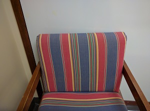
Let us take a look at this idea visually. Consider this image of a chair:
A visual representation of how this image is stored as a NumPy array is:
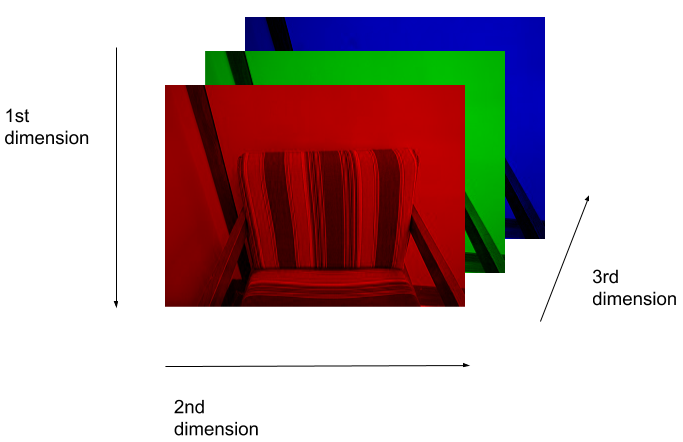
So, when we are working with skimage images, we specify the y coordinate first, then the x coordinate. And, the colors are stored as RGB values – red in layer 0, green in layer 1, blue in layer 2.
Coordinate and color channel order
CAUTION: it is vital to remember the order of the coordinates and color channels when dealing with images as NumPy arrays. If we are manipulating or accessing an image array directly, we specifiy the y coordinate first, then the x. Further, the first channel stored is the red channel, followed by the green, and then the blue.
Reading, displaying, and saving images
Skimage provides easy-to-use functions for reading, displaying, and saving images. All of the popular image formats, such as BMP, PNG, JPEG, and TIFF are supported, along with several more esoteric formats. See the skimage documentation for more information.
Let us examine a simple Python program to load, display, and save an image to a different format. Here are the first few lines:
"""
 * Python program to open, display, and save an image.
 *
"""
import skimage.io

# read image
image = skimage.io.imread(fname="chair.jpg")
First, we import the io module of skimage (skimage.io) so
we can read and write images. Then, we use the skimage.io.imread() function to read
a JPEG image entitled chair.jpg. Skimage reads the image, converts it from
JPEG into a NumPy array, and returns the array; we save the array in a variable
named image.
Next, we will do something with the image:
import skimage.viewer

# display image
viewer = skimage.viewer.ImageViewer(image)
viewer.show()
Once we have the image in the program, we next import the viewer module of skimage
(skimage.viewer) and display it using skimage.viewer.ImageViewer(), which
returns a ImageViewer object we store in the viewer variable.
We then call viewer.show() in order to display the image.
Next, we will save the image in another format:
# save a new version in .tif format
skimage.io.imsave(fname="chair.tif", arr=image)
The final statement in the program, skimage.io.imsave(fname="chair.tif", arr=image),
writes the image to a file named chair.tif. The imsave() function automatically
determines the type of the file, based on the file extension we provide. In
this case, the .tif extension causes the image to be saved as a TIFF.
Extensions do not always dictate file type
The skimage
imsave()function automatically uses the file type we specify in the file name parameter’s extension. Note that this is not always the case. For example, if we are editing a document in Microsoft Word, and we save the document aspaper.pdfinstead ofpaper.docx, the file is not saved as a PDF document.
Named versus positional arguments
When we call functions in Python, there are two ways we can specify the necessary arguments. We can specify the arguments positionally, i.e., in the order the parameters appear in the function definition, or we can use named arguments.
For example, the
skimage.io.imread()function definition specifies two parameters, the file name to read and an optional flag value. So, we could load in the chair image in the sample code above using positional parameters like this:
image = skimage.io.imread('chair.jpg')Since the function expects the first argument to be the file name, there is no confusion about what
'char.jpg'means.The style we will use in this workshop is to name each parameters, like this:
image = skimage.io.imsave(fname='chair.jpg')This style will make it easier for you to learn how to use the variety of functions we will cover in this workshop.
Resizing an image (20 min)
Using your mobile phone, tablet, web cam, or digital camera, take an image. Copy the image to the Desktop/workshops/image-processing/03-skimage-images directory. Write a Python program to read your image into a variable named
image. Then, resize the image by a factor of 50 percent, using this line of code:new_shape = (image.shape[0] // 2, image.shape[1] // 2, image.shape[2]) small = skimage.transform.resize(image=image, output_shape=new_shape)As it is used here, the parameters to the
skimage.transform.resize()function are the image to transform,image, the dimensions we want the new image to have.Finally, write the resized image out to a new file named resized.jpg. Once you have executed your program, examine the image properties of the output image and verify it has been resized properly.
Solution
Here is what your Python program might look like.
"""
 * Python program to read an image, resize it, and save it
 * under a different name.
"""
import skimage.io
import skimage.transform

# read in image
image = skimage.io.imread(fname="chicago.jpg")

# resize the image
new_shape = (image.shape[0] // 2, image.shape[1] // 2, image.shape[2])
small = skimage.transform.resize(image=image, output_shape=new_shape)

# write out image
skimage.io.imsave(fname="resized.jpg", arr=small)
From the command line, we would execute the program like this:
python Resize.pyThe program resizes the chicago.jpg image by 50% in both dimensions, and saves the result in the resized.jpg file.
Manipulating pixels
If we desire or need to, we can individually manipulate the colors of pixels by changing the numbers stored in the image’s NumPy array.
For example, suppose we are interested in this maize root cluster image. We want to be able to focus our program’s attention on the roots themselves, while ignoring the black background.
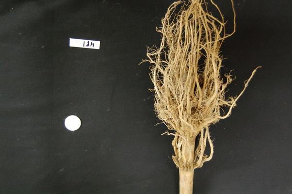
Since the image is stored as an array of numbers, we can simply look through the array for pixel color values that are less than some threshold value. This process is called thresholding, and we will see more powerful methods to perform the thresholding task in the Thresholding episode. Here, though, we will look at a simple and elegant NumPy method for thresholding. Let us develop a program that keeps only the pixel color values in an image that have value greater than or equal to 128. This will keep the pixels that are brighter than half of “full brightness;” i.e., pixels that do not belong to the black background. We will start by reading the image and displaying it.
"""
* Python script to ignore low intensity pixels in an image.
*
* usage: python HighIntensity.py <filename>
"""
import sys
import skimage.io
import skimage.viewer

# read input image, based on filename parameter
image = skimage.io.imread(fname=sys.argv[1])

# display original image
viewer = skimage.viewer.ImageViewer(image)
viewer.show()
Our program imports sys in addition to skimage, so that we can use
command-line arguments when we execute the program. In particular, in this
program we use a command-line argument to specify the filename of the image to
process. If the name of the file we are interested in is roots.jpg, and
the name of the program is HighIntensity.py, then we run our Python
program form the command line like this:
python HighIntensity.py roots.jpg
The place where this happens in the code is the
skimage.io.imread(fname=sys.argv[1])
function call. When we invoke our program with command line arguments,
they are passed in to the program as a list; sys.argv[1] is the first one
we are interested in; it contains the image filename we want to process.
(sys.argv[0] is simply the name of our program, HighIntensity.py in
this case).
Benefits of command-line arguments
Passing parameters such as filenames into our programs as parameters makes our code more flexible. We can now run HighIntensity.py on any image we wish, without having to go in and edit the code.
Now we can threshold the image and display the result.
# keep only high-intensity pixels
image[image < 128] = 0

# display modified image
viewer = skimage.viewer.ImageViewer(image)
viewer.show()
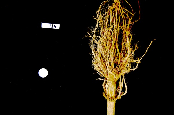
The NumPy command to ignore all low-intensity pixels is img[img < 128] = 0.
Every pixel color value in the whole 3-dimensional array with a value less
that 128 is set to zero. In this case, the result is an image in which the
extraneous background detail has been removed.
Keeping only low intensity pixels (20 min)
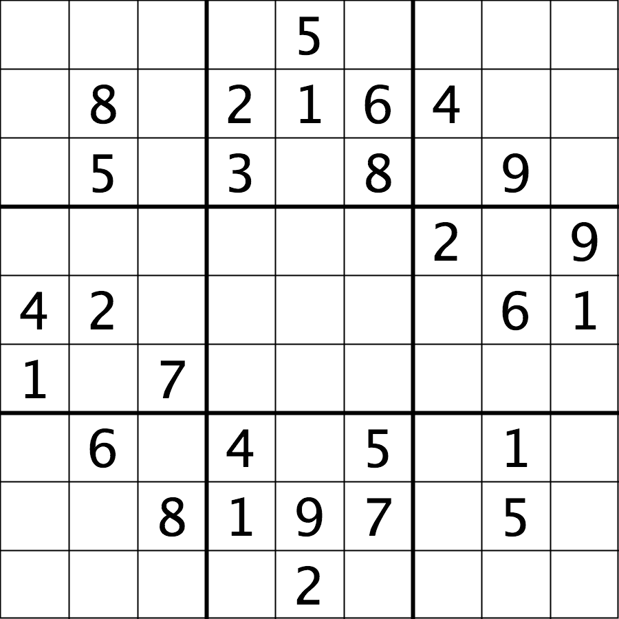
In the previous example, we showed how we could use Python and skimage to turn on only the high intensity pixels from an image, while turning all the low intensity pixels off. Now, you can practice doing the opposite – keeping all the low intensity pixels while changing the high intensity ones. Consider this image of a Su-Do-Ku puzzle, named sudoku.png:
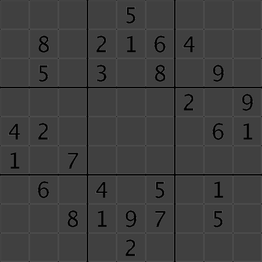
Navigate to the Desktop/workshops/image-processing/03-skimage-images directory, and copy the HighIntensity.py program to another file named LowIntensity.py. Then, edit the LowIntensity.py program so that it turns all of the white pixels in the image to a light gray color, say with all three color channel values for each formerly white pixel set to 64. Your results should look like this:
Solution
After modification, your program should look like this:
"""
* Python script to modify high intensity pixels in an image.
*
* usage: python LowIntensity.py <filename>
"""
import sys
import skimage.io
import skimage.viewer

# read input image, based on filename parameter
img = skimage.io.imread(fname=sys.argv[1])

# display original image
viewer = skimage.viewer.ImageViewer(img)
viewer.view()

# change high intensity pixels to gray
img[img > 200] = 64

# display modified image
viewer = skimage.viewer.ImageViewer(img)
viewer.view()
Converting color images to grayscale
It is often easier to work with grayscale images, which have a single channel,
instead of color images, which have three channels.
Skimage offers the function skimage.color.rgb2gray() to achieve this.
This function adds up the three color channels in a way that matches
human color perception, see the skimage documentation for details.
It returns a grayscale image with floating point values in the range from 0 to 1.
We can use the function skimage.util.img_as_ubyte() in order to convert it back to the
original data type and the data range back 0 to 255.
Note that it is often better to use image values represented by floating point values,
because using floating point numbers is numerically more stable.
"""
* Python script to load a color image as grayscale.
*
* usage: python LoadGray.py <filename>
"""
import sys
import skimage.io
import skimage.viewer
import skimage.color

# read input image, based on filename parameter
image = skimage.io.imread(fname=sys.argv[1])

# display original image
viewer = skimage.viewer.ImageViewer(image)
viewer.show()

# convert to grayscale and display
gray_image = skimage.color.rgb2gray(image)
viewer = skimage.viewer.ImageViewer(gray_image)
viewer.show()
We can also load color images as grayscale directly by passing the argument as_gray=True to
skimage.io.imread().
"""
* Python script to load a color image as grayscale.
*
* usage: python LoadGray.py <filename>
"""
import sys
import skimage.io
import skimage.viewer
import skimage.color

# read input image, based on filename parameter
image = skimage.io.imread(fname=sys.argv[1], as_gray=True)

# display grayscale image
viewer = skimage.viewer.ImageViewer(image)
viewer.show()
Access via slicing
Since skimage images are stored as NumPy arrays, we can use array slicing to select rectangular areas of an image. Then, we could save the selection as a new image, change the pixels in the image, and so on. It is important to remember that coordinates are specified in (y, x) order and that color values are specified in (r, g, b) order when doing these manipulations.
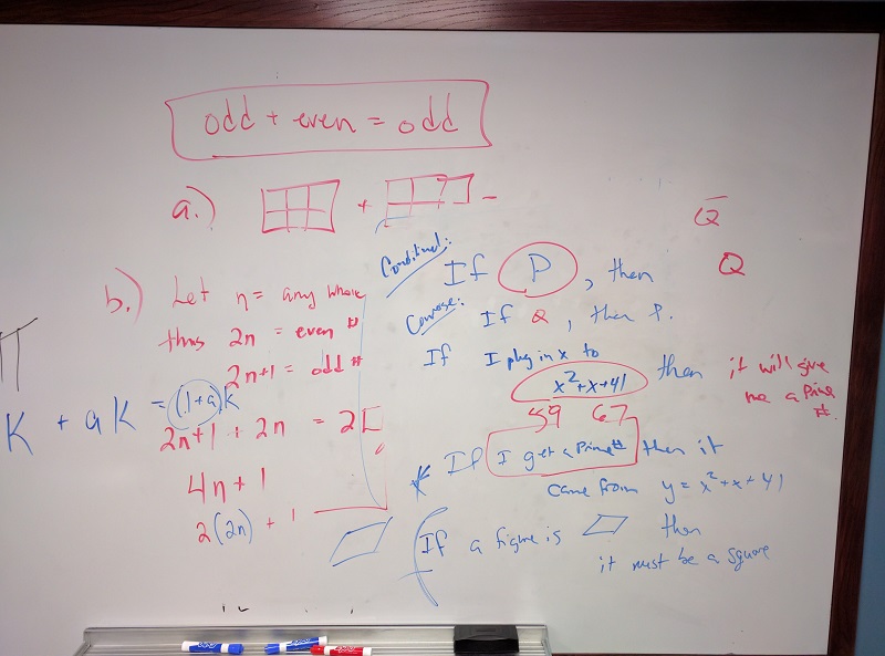
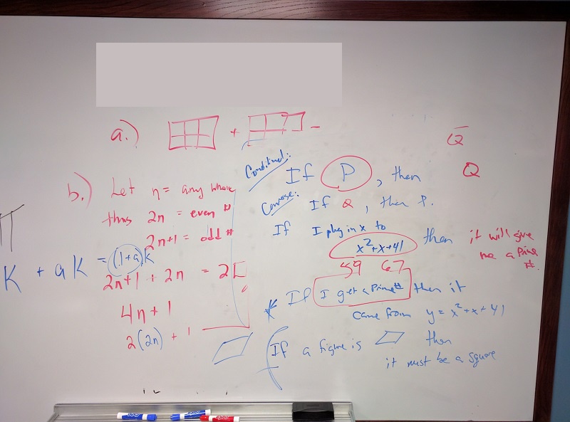
Consider this image of a whiteboard, and suppose that we want to create a sub-image with just the portion that says “odd + even = odd,” along with the red box that is drawn around the words.
We can use a tool such as ImageJ to determine the coordinates of the corners of the area we wish to extract. If we do that, we might settle on a rectangular area with an upper-left coordinate of (135, 60) and a lower-right coordinate of (480, 150), as shown in this version of the whiteboard picture:
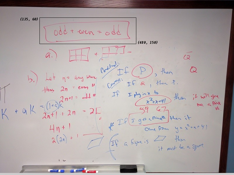
Note that the coordinates in the preceding image are specified in (x, y)
order. Now if our entire whiteboard image is stored as an skimage image named
image, we can create a new image of the selected region with a statement like
this:
clip = image[60:151, 135:481, :]
Our array slicing specifies the range of y-coordinates first, 60:151, and
then the range of x-coordinates, 135:481. Note we go one beyond the maximum
value in each dimension, so that the entire desired area is selected.
The third part of the slice, :, indicates that we want all three color
channels in our new image.
A program to create the subimage would start by loading the image:
"""
 * Python script demonstrating image modification and creation via
 * NumPy array slicing.
"""
import skimage.io
import skimage.viewer

# load and display original image
image = skimage.io.imread(fname="board.jpg")
viewer = skimage.viewer.ImageViewer(image)
viewer.show()
Then we use array slicing to create a new image with our selected area and then display the new image.
# extract, display, and save sub-image
clip = image[60:151, 135:481, :]
viewer = skimage.viewer.ImageViewer(clip)
viewer.show()
skimage.io.imsave(fname="clip.tif", arr=clip)
We can also change the values in an image, as shown next.
# replace clipped area with sampled color
color = image[330, 90]
image[60:151, 135:481] = color
viewer = skimage.viewer.ImageViewer(image)
viewer.show()
First, we sample the color at a particular location of the
image, saving it in a NumPy array named color, a 1 × 1 × 3 array with the blue,
green, and red color values for the pixel located at (x = 90, y = 330). Then,
with the img[60:151, 135:481] = color command, we modify the image in the
specified area. In this case, the command “erases” that area of the whiteboard,
replacing the words with a white color, as shown in the final image produced by
the program:
Practicing with slices (10 min)
Navigate to the Desktop/workshops/image-processing/03-skimage-images directory, and edit the RootSlice.py program. It contains a skeleton program that loads and displays the maize root image shown above. Modify the program to create, display, and save a sub-image containing only the plant and its roots. Use ImageJ to determine the bounds of the area you will extract using slicing.
Solution
Here is the completed Python program to select only the plant and roots in the image.
"""
 * Python script to extract a sub-image containing only the plant and
 * roots in an existing image.
"""
import skimage.io
import skimage.viewer

# load and display original image
image = skimage.io.imread(fname="roots.jpg")
viewer = skimage.viewer.ImageViewer(image)
viewer.show()

# extract, display, and save sub-image
# WRITE YOUR CODE TO SELECT THE SUBIMAGE NAME clip HERE:
clip = image[0:1999, 1410:2765, :]
viewer = skimage.viewer.ImageViewer(clip)
viewer.show()


# WRITE YOUR CODE TO SAVE clip HERE
skimage.io.imsave(fname="clip.jpg", arr=clip)
Metadata, continued (10 min)
Let us return to the concept of image metadata, introduced briefly in the Image Basics episode. Specifically, what happens to the metadata of an image when it is read into, and written from, a Python program using skimage?
To answer this question, write a very short (three lines) Python script to read in a file and save it under a different name. Navigate to the Desktop/workshops/image-processing/03-skimage-images directory, and write your script there. You can use the flowers-before.jpg as input, and save the output as flowers-after.jpg. Then, examine the metadata from both images using commands like identify -verbose flowers-after.jpg. Is the metadata the same? If not, what are some key differences?
Solution
Here is a short Python script to open the image and save it in a different filename:
import skimage.io

img = skimage.io.imread(fname="flowers-before.jpg")
skimage.io.imsave(fname="flowers-after.jpg", arr=img)
The newly-saved file is missing most of the original metadata. Comparing this to the original, as shown in the Image Basics episode, it is easy to see that virtually all of the useful metadata has been lost!
The moral of this challenge is to remember that image metadata will not be preserved in images that your programs write via the
skimage.io.imsave()function. If metadata is important to you, take precautions to always preserve the original files.
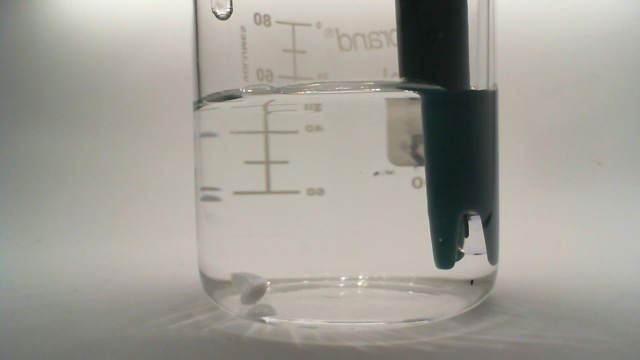
Slicing and the colorimetric challenge (10 min)
In the introductory episode, we were introduced to a colorimetric challenge, namely, graphing the color values of a solution in a titration, to see when the color change takes place. Let’s start thinking about how to solve that problem.
One part of our ultimate solution will be sampling the color channel values from an image of the solution. To make our graph more reliable, we will want to calculate a mean channel value over several pixels, rather than simply focusing on one pixel from the image.
Navigate to the Desktop/workshops/image-processing/10-challenges/colorimetrics directory, and open the titration.tiff image in ImageJ.
Find the (x, y) coordinates of an area of the image you think would be good to sample in order to find the average channel values. Then, write a small Python program that computes the mean channel values for a 10 × 10 pixel kernel centered around the coordinates you chose. Print the results to the screen, in a format like this:
Avg. red value: 193.7778
Avg. green value: 189.1481
Avg. blue value: 178.6049
Key Points
skimage images are stored as three-dimensional NumPy arrays.
In skimage images, the red channel is specified first, then the green, then the blue, i.e. RGB.
Images are read from disk with the
skimage.io.imread()function.We create a window that automatically scales the displayed image with
skimage.viewer.ImageViewer()and callingview()on the viewer object.Color images can be transformed to grayscale using
skimage.color.rgb2gray()or be read as grayscale directly by passing the argumentas_gray=Truetoskimage.io.imread().We can resize images with the
skimage.transform.resize()function.NumPy array commands, like
img[img < 128] = 0, and be used to manipulate the pixels of an image.Command-line arguments are accessed via the
sys.argvlist;sys.argv[1]is the first parameter passed to the program,sys.argv[2]is the second, and so on.Array slicing can be used to extract sub-images or modify areas of images, e.g.,
clip = img[60:150, 135:480, :].Metadata is not retained when images are loaded as skimage images.