Overview

Teaching: ?? min
Exercises: ?? min

Questions

• How to extract separate objects from an image and describe these objects quantitatively.

Objectives

• Understand the term object in the context of images.

• Learn about pixel connectivity.

• Learn how Connected Component Analysis (CCA) works.

• Use CCA to produce an image that highlights every object in a different color.

• Characterize each object with numbers that describe its appearance.

Objects

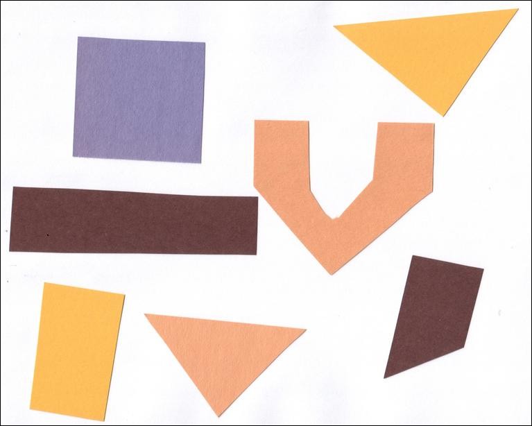
In the thresholding episode we have covered dividing an image in foreground and background pixels. In the junk example image, we considered the colored shapes as foreground objects on a white background.

In thresholding we went from the original image to this version:

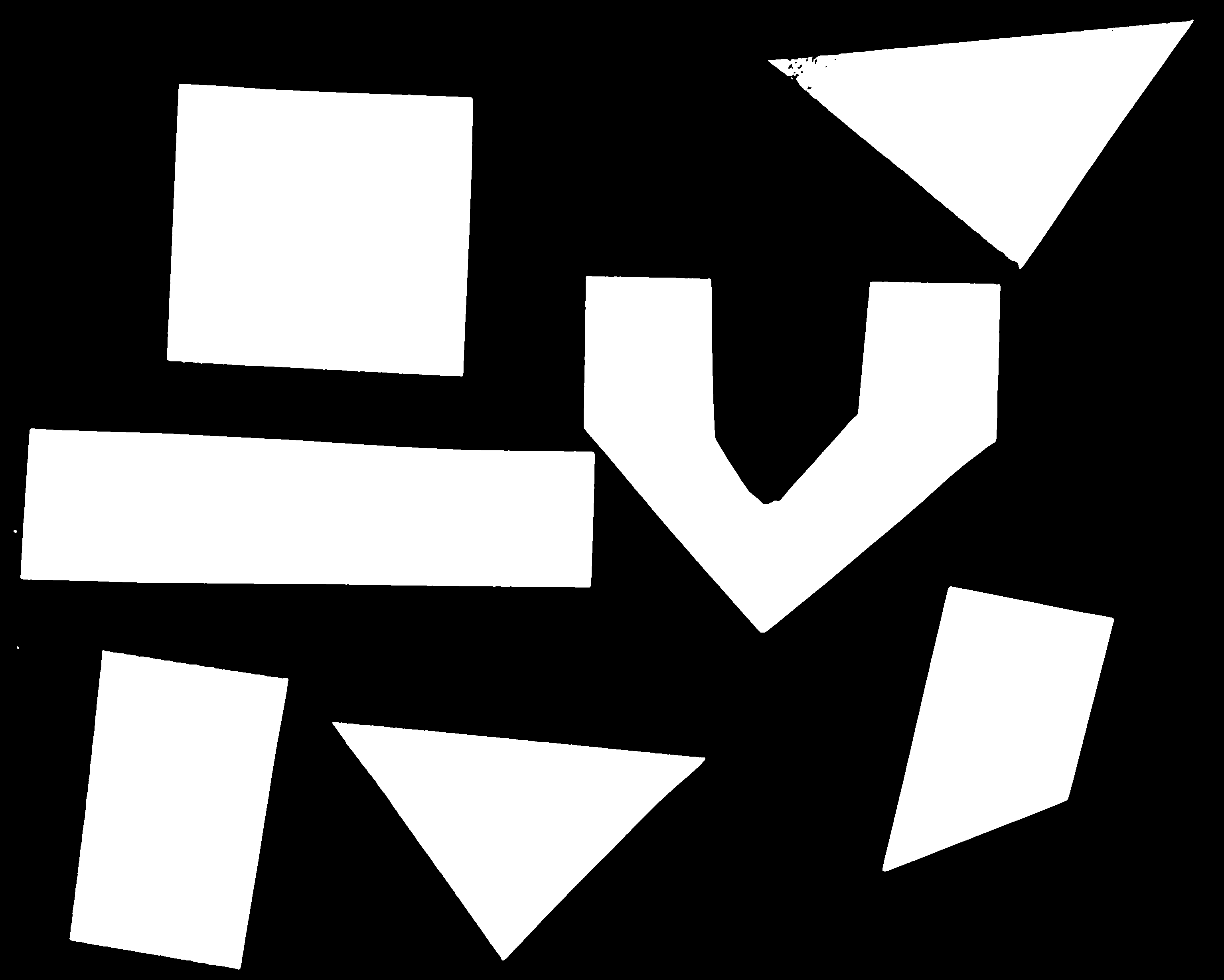
Here, we created a mask that only highlights the parts of the image that we find interesting, the objects. All objects have pixel value of True while the background pixels are False.

By looking at the mask image, one can count the objects that are present in the image (7). But how did we actually do that, how did we decide which lump of pixels constitutes a single object?

Pixel Neighborhoods

In order to decide which pixels belong to the same object, one can exploit their neighbourhood: pixels that are directly next to each other and belong to the foreground class can be considered to belong to the same object.

Let’s consider the following mask “image” with 8 rows, and 8 columns. Note that for brevity, 0 is used to represent False (background) and 1 to represent True (foreground).

0 0 0 0 0 0 0 0
0 1 1 0 0 0 0 0
0 1 1 0 0 0 0 0
0 0 0 1 1 1 0 0
0 0 0 1 1 1 1 0
0 0 0 0 0 0 0 0

The pixels are organized in a rectangular grid. In order to understand pixel neighborhoods we will introduce the concept of “jumps” between pixels. The jumps follow two rules: First rule is that one jump is only allowed along the column, or the row. Diagonal jumps are not allowed. So, from a center pixel, denoted with o, only the pixels indicated with an x are reachable:

- x -
x o x
- x -

The pixels on the diagonal (from o) are not reachable with a single jump, which is denoted by the -. The pixels reachable with a single jump form the 1-jump neighborhood.

The second rule states that in a sequence of jumps, one may only jump in row and column direction once -> they have to be orthogonal. An example of a sequence of orthogonal jumps is shown below. Starting from o the first jump goes along the row to the right. The second jump then goes along the column direction up. After this the sequence cannot be continued as a jump has been made in row and column direction.

- - 2
- o 1
- - -

All pixels reachable with one, or two jumps form the 2-jump neighborhood. The grid below illustrates the pixels reachable from the center pixel o with a single jump, highlighted with a 1, and the pixels reachable with 2 jumps with a 2.

2 1 2
1 o 1
2 1 2

We want to revisiting our example image mask from above and apply the two different neighborhood rules. With a single jump connectivity for each pixel, we get two resulting objects, highlighted in the image with 1’s and 2’s.

0 0 0 0 0 0 0 0
0 1 1 0 0 0 0 0
0 1 1 0 0 0 0 0
0 0 0 2 2 2 0 0
0 0 0 2 2 2 2 0
0 0 0 0 0 0 0 0

In the 1-jump version, only pixels that neighbors in rows or columns, are considered connected. With two jumps, however, we only get a single objects, as pixels are also considered connected along the diagonals.

0 0 0 0 0 0 0 0
0 1 1 0 0 0 0 0
0 1 1 0 0 0 0 0
0 0 0 1 1 1 0 0
0 0 0 1 1 1 1 0
0 0 0 0 0 0 0 0

Exercise: Object counting

How many objects with 1 orthogonal jump, how many with 2 orthogonal jumps?

0 0 0 0 0 0 0 0
0 1 0 0 0 1 1 0
0 0 1 0 0 0 0 0
0 1 0 1 1 1 0 0
0 1 0 1 1 0 0 0
0 0 0 0 0 0 0 0

1 jump

a) 1 b) 5 c) 2

Solution

b) 5

2 jumps

a) 2 b) 3 c) 5

Solution

a) 2

Jumps and neighborhoods

We have just introduced how you can reach different neighboring pixels by performing one or more orthogonal jumps. There is also a different way of referring to these pixels: the 4- and 8-neighborhood. With a single jump you can reach four pixels from a given starting pixel. Hence, the one jump neighborhood corresponds to the 4-neighborhood. When two orthogonal jumps are allowed, eight pixels can be reached, so this corresponds to the 8-neighborhood.

Connected Component Analysis

In order to find the objects in an image, we want to employ an operation that is called Connected Component Analysis (CCA). This operation takes a binary image as an input. Usually, the False value in this image is associated with background pixels, and the True value indicates foreground, or object pixels. Such an image can be e.g. produced with thresholding. Given a thresholded image, CCA produces a new labeled image with integer pixel values. Pixels with the same value, belong to the same object.

We use the thresholding script as a starting point to write a program, that prints the number of objects in an image.

"""
 * Python script count objects in an image
 *
 * usage: python CCA.py <filename> <sigma> <threshold>
"""
import sys
import numpy as np
import skimage.color
import skimage.filters
import skimage.io
import skimage.viewer
import skimage.measure
import skimage.color

# get filename, sigma, and threshold value from command line
filename = sys.argv[1]
sigma = float(sys.argv[2])
t = float(sys.argv[3])

# read and display the original image
image = skimage.io.imread(fname=filename, as_gray=True)
viewer = skimage.viewer.ImageViewer(image)
viewer.show()

# blur and grayscale before thresholding
blur = skimage.filters.gaussian(image, sigma=sigma)

# perform inverse binary thresholding
mask = blur < t

# display the result
viewer = skimage.viewer.ImageViewer(mask)
viewer.show()

# Perform CCA on the mask
labeled_image = skimage.measure.label(mask, connectivity=2, return_num=True)

viewer = skimage.viewer.ImageViewer(labeled_image)
viewer.show()

Let’s examine the changes to the original thresholding script. There is an additional import: skimage.measure. We import skimage.measure in order to use the skimage.measure.label function that performs CCA.

After the imports, the parameters for sigma and the threshold are read from the command line. The original image is displayed first, then blurring and thresholding is performed. The resulting binary image is also displayed in an interactive viewer. The new code follows the comment Perform CCA on the mask. The skimage function to perform CCA is skimage.measure.label. It has one positional argument, where we supply mask, the binary image to work on. With an optional argument we, specify the connectivity in units of orthogonal jumps. By setting connectivity=2 we will consider a particular pixel connected to a second one, if the second one is reachable with two orthogonal jumps from the first pixel. The function returns an image in which each object is represented with a unique pixel value. We assign this image to the variable labeled_image.

Calling the script with the junk.jpg image and sigma=2.0 and threshold=0.9 yields an all black image. Note: this behavior might change in future versions, or not occur with a different image viewer.

What went wrong?

When we hover with the mouse over this black image, the underlying pixel values are shown as numbers in the lower left corner. We can see that in some positions they are not 0, but still this image is black.

Let’s find out more by examining label_image. Properties that might be interesting in this context are dtype, the minimum and maximum value. We can do so by adding the following lines:

print("dtype:", label_image.dtype)
print("min:", numpy.min(label_image))
print("max:", numpy.max(label_image))

Examining the output can give us a clue:

dtype: int64
min: 0
max: 11

The dtype of label_image is int64. This means that values in this image range from -2 ** 63 to 2 ** 63 - 1. Those are really big numbers. From this available space we only use the range from 0 to 11. When showing this image in the viewer, it squeezes the complete range into 256 gray values. The range of our numbers does not produce any visible change. The skimage library has tools to cope with this a situation. In the skimage.color module has a function label2rgb() that will do the conversion. We have already used the skimage.color module to convert color images to gray scale images. skimage.color.label2rgb() will create a new color image. All objects are colored according to a list of colors that can be customized. In order to see our objects, we can add the following code to our program:

# convert the label image to color image
colored_label_image = skimage.color.label2rgb(labeled_image, bg_label=0)

# show the created image in the viewer
viewer = skimage.viewer.ImageViewer(colored_label_image)
viewer.show()

How many objects are in that image (15 min)

Now, it is your turn to practice. Using the original junk.png image, copy the CCA.py script to a new file CCA-count.py. Modify this script to print out the number of found objects in the end.

What number of objects would you expect to get? How does changing the sigma and threshold values influence the result?

Solution

All pixels that belong to a single object are assigned the same integer value. The algorithm produces consecutive numbers. That means the first object gets the value 1, the second object the value 2 and so on. This means that, by finding the object with the maximum value, we know how many objects there are in the image. Using the numpy.max function will give us the maximum value in the image

Adding the following code at the end of the CCA-count.py program will print out the number of objects

num_objects = numpy.max(labeled_image)
print("Found", num_objects, "objects in the image.")

Invoking the program with sigma=2.0, and threshold=0.9 will print

Found 11 objects in the image.

Lowering the threshold will result in fewer objects. The higher the threshold is set, the more objects are found. More and more background noise gets picked up as objects.

Larger sigmas produce binary masks with less noise and hence a smaller number of objects. Setting sigma too high bears the danger of merging objects.

Morphometrics - Describe object features with numbers

Plot a histogram of the object area distribution (15 min)

In the previous exercise we wrote the CCA-count.py program and explored how the object count changed with the parameters. We had a hard time making the script print out the right number of objects. In order to get closer to a solution to this problem, we want to look at the distribution of the object areas. Calculate the object properties using skimage.measure.regionprops and generate a histogram.

Make a copy of the CCA.py script and modify it to also produce a plot of the histogram of the object area.

What does the histogram tell you about the objects?

Hint: Try to generate a list of object areas first.

Solution

# add the import for pyplot
from matplotlib import pyplot as plt

# compute object features and extrac object areas
object_features = skimage.measure.regionprops(labeled_image)
object_areas = [objf["area"] for objf in object_features]
plt.hist(object_areas)
plt.show()

Filter objects by area (15 min)

Our CCA-count.py program has an apparent problem: it is hard to find a combination that produces the right output number. In some cases the problem arose that some background noise got picked up as an object. With other parameter settings some of the foreground objects got broken up or disappeared completely.

Modify the program in order to only count large objects.

Solution

Now make this change visual: Modify the label image such that objects below a certain area are set to the background label (0).

Solution

# iterate over object_ids and modify the `labeled_image` in-place
for object_id, objf in enumerate(object_features, start=1):
    if objf["area"] < 10000:
        labeled_image[labeled_image == object_id] = 0

Lastly print out the count for the large objects

Solution

# generate a list of objects above a certain area
filtered_list = []
for objf in object_features:
    if objf["area"] > 10000:
        filtered_list.append(objf["area"])

print("Found", len(filtered_list), "objects!")

The script, if working properly, will produce the following output:

Fount 7 objects!

Key Points

• skimage.measure.label is used to generate objects.

• We use skimage.measure.regionprops to measure properties of labelled objects.

• Color objects according to feature values.