Image Basics
Overview
Teaching: 35 min
Exercises: 15 minQuestions
How are images represented in digital format?
Objectives
Define the terms bit, byte, kilobyte, megabyte, etc.
Explain how a digital image is composed of pixels.
Explain the left-hand coordinate system used in digital images.
Explain the RGB additive color model used in digital images.
Explain the characteristics of the BMP, JPEG, and TIFF image formats.
Explain the difference between lossy and lossless compression.
Explain the advantages and disadvantages of compressed image formats.
Explain what information could be contained in image metadata.
The images we see on hard copy, view with our electronic devices, or process with our programs are represented and stored in the computer as numeric abstractions, approximations of what we see with our eyes in the real world. Before we begin to learn how to process images with Python programs, we need to spend some time understanding how these abstractions work.
Bits and bytes
Before we talk specifically about images, we first need to understand how numbers are stored in a modern digital computer. When we think of a number, we do so using a decimal, or base-10 place-value number system. For example, a number like 659 is 6 × 10² + 5 × 101 + 9 × 100. Each digit in the number is multiplied by a power of 10, based on where it occurs, and there are 10 digits that can occur in each position (0, 1, 2, 3, 4, 5, 6, 7, 8, 9).
In principle, computers could be constructed to represent numbers in exactly the same way. But, as it turns out, the electronic circuits inside a computer are much easier to construct if we restrict the numeric base to only two, versus 10. (It is easier for circuitry to tell the difference between two voltage levels than it is to differentiate between 10 levels.) So, values in a computer are stored using a binary, or base-2 place-value number system.
In this system, each symbol in a number is called a bit instead of a digit, and there are only two values for each bit (0 and 1). We might imagine a four-bit binary number, 1101. Using the same kind of place-value expansion as we did above for 659, we see that 1101 = 1 × 23 + 1 × 22 + 0 × 21 + 1 × 20, which if we do the math is 8 + 4 + 0 + 1, or 13 in decimal.
Internally, computers have a minimum number of bits that they work with at a given time: eight. A group of eight bits is called a byte. The amount of memory (RAM) and drive space our computers have is quantified by terms like Megabytes (MB), Gigabytes (GB), and Terabytes (TB). The following table provides more formal definitions for these terms.
| Unit | Abbreviation | Size |
|---|---|---|
| Kilobyte | KB | 1024 bytes |
| Megabyte | MB | 1024 KB |
| Gigabyte | GB | 1024 MB |
| Terabyte | TB | 1024 GB |
Pixels
It is important to realize that images are stored as rectangular arrays of hundreds, thousands, or millions of discrete “picture elements,” otherwise known as pixels. Each pixel can be thought of as a single square point of colored light.
For example, consider this image of a maize seedling, with a square area designated by a red box:
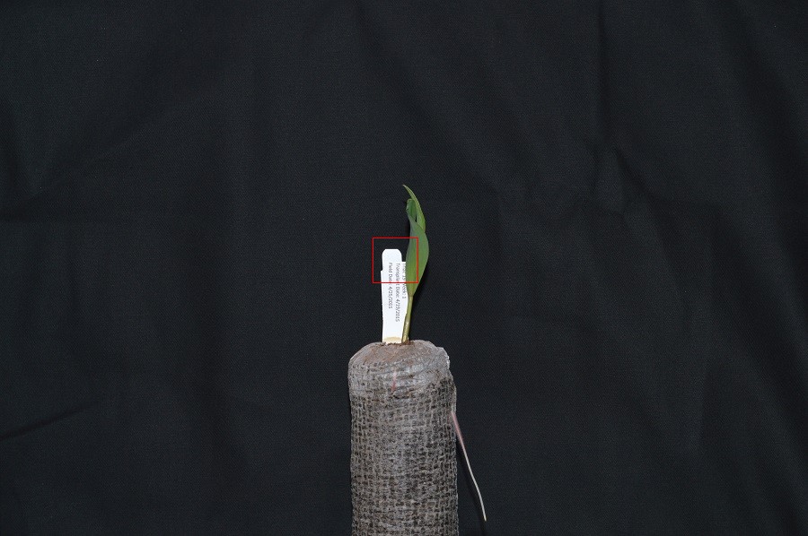
Now, if we zoomed in close enough to see the pixels in the red box, we would see something like this:
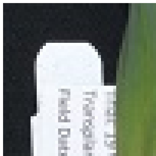
Note that each square in the enlarged image area – each pixel – is all one color, but that each pixel can have a different color from its neighbors. Viewed from a distance, these pixels seem to blend together to form the image we see.
Coordinate system
When we process images, we can access, examine, and / or change the color of any pixel we wish. To do this, we need some convention on how to access pixels individually; a way to give each one a name, or an address of a sort.
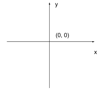
The most common manner to do this, and the one we will use in our programs, is to assign a modified Cartesian coordinate system to the image. The coordinate system we usually see in mathematics has a horizontal x-axis and a vertical y-axis, like this:
The modified coordinate system used for our images will have only positive coordinates, the origin will be in the upper left corner instead of the center, and y coordinate values will get larger as they go down instead of up, like this:
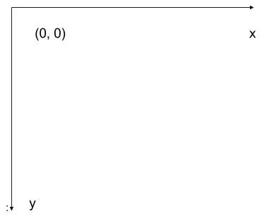
This is called a left-hand coordinate system. If you hold your left hand in front of your face and point your thumb at the floor, your extended index finger will correspond to the x-axis while your thumb represents the y-axis.
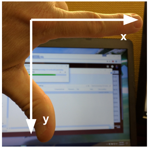
Until you have worked with images for a while, the most common mistake that you will make with coordinates is to forget that y coordinates get larger as they go down instead of up as in a normal Cartesian coordinate system.
Color model
Digital images use some color model to create a broad range of colors from a small set of primary colors. Although there are several different color models that are used for images, the most commonly occurring one is the RGB (Red, Green, Blue) model.
The RGB model is an additive color model, which means that the primary colors are mixed together to form other colors. In the RGB model, the primary colors are red, green, and blue – thus the name of the model. Each primary color is often called a channel.
Most frequently, the amount of the primary color added is represented as an integer in the closed range [0, 255]. Therefore, there are 256 discrete amounts of each primary color that can be added to produce another color. The number of discrete amounts of each color, 256, corresponds to the number of bits used to hold the color channel value, which is eight (28=256). Since we have three channels, this is called 24-bit color depth.
Any particular color in the RGB model can be expressed by a triplet of integers in [0, 255], representing the red, green, and blue channels, respectively. A larger number in a channel means that more of that primary color is present.
Thinking about RGB colors (3 min)
Suppose that we represent colors as triples (r, g, b), where each of r, g, and b is an integer in [0, 255]. What colors are represented by each of these triples? (Try to answer these questions without reading further.)
- (255, 0, 0)
- (0, 255, 0)
- (0, 0, 255)
- (255, 255, 255)
- (0, 0, 0)
- (128, 128, 128)
Solution
- (255, 0, 0) represents red, because the red channel is maximized, while the other two channels have the minimum values.
- (0, 255, 0) represents green.
- (0, 0, 255) represents blue.
- (255, 255, 255) is a little harder. When we mix the maximum value of all three color channels, we see the color white.
- (0, 0, 0) represents the absence of all color, or black.
- (128, 128, 128) represents a medium shade of gray. Note that the 24-bit RGB color model provides at least 254 shades of gray, rather than only fifty.
Note that the RGB color model may run contrary to your experience, especially if you have mixed primary colors of paint to create new colors. In the RGB model, the lack of any color is black, while the maximum amount of each of the primary colors is white. With physical paint, we might start with a white base, and then add differing amounts of other paints to produce a darker shade.
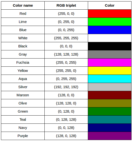
After completing the previous challenge, we can look at some further examples of 24-bit RGB colors, in a visual way. The image in the next challenge shows some color names, their 24-bit RGB triplet values, and the color itself.
RGB color table (4 min)
We cannot really provide a complete table. To see why, answer this question: How many possible colors can be represented with the 24-bit RGB model?
Solution
There are 24 total bits in an RGB color of this type, and each bit can be on or off, and so there are 224 = 16,777,216 possible colors with our additive, 24-bit RGB color model.
Although 24-bit color depth is common, there are other options. We might have 8-bit color (3 bits for red and green, but only 2 for blue, providing 8 × 8 × 4 = 256 colors) or 16-bit color (4 bits for red, green, and blue, plus 4 more for transparency, providing 16 × 16 × 16 = 4096 colors), for example. There are color depths with more than eight bits per channel, but as the human eye can only discern approximately 10 million different colors, these are not often used.
If you are using an older or inexpensive laptop screen or LCD monitor to view images, it may only support 18-bit color, capable of displaying 64 × 64 × 64 = 262,144 colors. 24-bit color images will be converted in some manner to 18-bit, and thus the color quality you see will not match what is actually in the image.
We can combine our coordinate system with the 24-bit RGB color model to gain a conceptual understanding of the images we will be working with. An image is a rectangular array of pixels, each with its own coordinate. Each pixel in the image is a square point of colored light, where the color is specified by a 24-bit RGB triplet. Such an image is an example of raster graphics.
Image formats
Although the images we will manipulate in our programs are conceptualized as rectangular arrays of RGB triplets, they are not necessarily created, stored, or transmitted in that format. There are several image formats we might encounter, and we should know the basics of at least of few of them. Some formats we might encounter, and their file extensions, are shown in this table:
| Format | Extension |
|---|---|
| Device-Independent Bitmap (BMP) | .bmp |
| Joint Photographic Experts Group (JPEG) | .jpg or .jpeg |
| Tagged Image File Format (TIFF) | .tif or .tiff |
BMP
The file format that comes closest to our preceding conceptualization of images is the Device-Independent Bitmap, or BMP, file format. BMP files store raster graphics images as long sequences of binary-encoded numbers that specify the color of each pixel in the image. Since computer files are one-dimensional structures, the pixel colors are stored one row at a time. That is, the first row of pixels (those with y-coordinate 0) are stored first, followed by the second row (those with y-coordinate 1), and so on. Depending on how it was created, a BMP image might have 8-bit, 16-bit, or 24-bit color depth.
24-bit BMP images have a relatively simple file format, can be viewed and loaded across a wide variety of operating systems, and have high quality. However, BMP images are not compressed, resulting in very large file sizes for any useful image resolutions.
The idea of image compression is important to us for two reasons: first, compressed images have smaller file sizes, and are therefore easier to store and transmit; and second, compressed images may not have as much detail as their uncompressed counterparts, and so our programs may not be able to detect some important aspect if we are working with compressed images. Since compression is important to us, we should take a brief detour and discuss the concept.
Image compression
Let’s begin our discussion of compression with a simple challenge.
BMP image size (8 min)
Imagine that we have a fairly large, but very boring image: a 5,000 × 5,000 pixel image composed of nothing but white pixels. If we used an uncompressed image format such as BMP, with the 24-bit RGB color model, how much storage would be required for the file?
Solution
In such an image, there are 5,000 × 5,000 = 25,000,000 pixels, and 24 bits for each pixel, leading to 25,000,000 × 24 = 600,000,000 bits, or 75,000,000 bytes (71.5MB). That is quite a lot of space for a very uninteresting image!
Since image files can be very large, various compression schemes exist for saving (approximately) the same information while using less space. These compression techniques can be categorized as lossless or lossy.
Lossless compression
In lossless image compression, we apply some algorithm (i.e., a computerized procedure) to the image, resulting in a file that is significantly smaller than the uncompressed BMP file equivalent would be. Then, when we wish to load and view or process the image, our program reads the compressed file, and reverses the compression process, resulting in an image that is identical to the original. Nothing is lost in the process – hence the term “lossless.”
The general idea of lossless compression is to somehow detect long patterns of bytes in a file that are repeated over and over, and then assign a smaller bit pattern to represent the longer sample. Then, the compressed file is made up of the smaller patterns, rather than the larger ones, thus reducing the number of bytes required to save the file. The compressed file also contains a table of the substituted patterns and the originals, so when the file is decompressed it can be made identical to the original before compression.
To provide you with a concrete example, consider the 71.5 MB white BMP image discussed above. When put through the zip compression utility on Microsoft Windows, the resulting .zip file is only 72 KB in size! That is, the .zip version of the image is three orders of magnitude smaller than the original, and it can be decompressed into a file that is byte-for-byte the same as the original. Since the original is so repetitious – simply the same color triplet repeated 25,000,000 times – the compression algorithm can dramatically reduce the size of the file.
If you work with .zip or .gz archives, you are dealing with lossless compression.
Lossy compression
Lossy compression takes the original image and discards some of the detail in it, resulting in a smaller file format. The goal is to only throw away detail that someone viewing the image would not notice. Many lossy compression schemes have adjustable levels of compression, so that the image creator can choose the amount of detail that is lost. The more detail that is sacrificed, the smaller the image files will be – but of course, the detail and richness of the image will be lower as well.
This is probably fine for images that are shown on Web pages or printed off on 4 × 6 photo paper, but may or may not be fine for scientific work. You will have to decide whether the loss of image quality and detail are important to your work, versus the space savings afforded by a lossy compression format.
It is important to understand that once an image is saved in a lossy compression format, the lost detail is just that – lost. I.e., unlike lossless formats, given an image saved in a lossy format, there is no way to reconstruct the original image in a byte-by-byte manner.
JPEG
JPEG images are perhaps the most commonly encountered digital images today. JPEG uses lossy compression, and the degree of compression can be tuned to your liking. It supports 24-bit color depth, and since the format is so widely used, JPEG images can be viewed and manipulated easily on all computing platforms.
Examining actual image sizes (5 min)
Let us see the effects of image compression on image size with actual images. Open a terminal and navigate to the Desktop/workshops/image-processing/02-image-basics directory. This directory contains a simple program, ws.py that creates a square white image of a specified size, and then saves it as a BMP and as a JPEG image.
To create a 5,000 x 5,000 white square, execute the program by typing python ws.py 5000 and then hitting enter. Then, examine the file sizes of the two output files, ws.bmp and ws.jpg. Does the BMP image size match our previous prediction? How about the JPEG?
Solution
The BMP file, ws.bmp, is 75,000,054 bytes, which matches our prediction very nicely. The JPEG file, ws.jpg, is 392,503 bytes, two orders of magnitude smaller than the bitmap version.
Comparing lossless versus lossy compression (8 min)
Let us see a hands-on example of lossless versus lossy compression. Once again, open a terminal and navigate to the Desktop/workshops/image-processing/02-image-basics directory. The two output images, ws.bmp and ws.jpg, should still be in the directory, along with another image, tree.jpg.
We can apply lossless compression to any file by using the zip command. Recall that the ws.bmp file contains 75,000,054 bytes. Apply lossless compression to this image by executing the following command: zip ws.zip ws.bmp. This command tells the computer to create a new compressed file, ws.zip, from the original bitmap image. Execute a similar command on the tree JPEG file: zip tree.zip tree.jpg.
Having created the compressed file, use the ls -al command to display the contents of the directory. How big are the compressed files? How do those compare to the size of ws.bmp and tree.jpg? What can you conclude from the relative sizes?
Solution
Here is a partial directory listing, showing the sizes of the relevant files there:
-rw-rw-r– 1 diva diva 154344 Jun 18 08:32 tree.jpg
-rw-rw-r– 1 diva diva 146049 Jun 18 08:53 tree.zip
-rw-rw-r– 1 diva diva 75000054 Jun 18 08:51 ws.bmp
-rw-rw-r– 1 diva diva 72986 Jun 18 08:53 ws.zip
We can see that the regularity of the bitmap image (remember, it is a 5,000 x 5,000 pixel image containing only white pixels) allows the lossless compression scheme to compress the file quite effectively. On the other hand, compressing tree.jpg does not create a much smaller file; this is because the JPEG image was already in a compressed format.
Here is an example showing how JPEG compression might impact image quality. Consider this image of several maize seedlings (scaled down here from 11,339 × 11,336 pixels in order to fit the display).
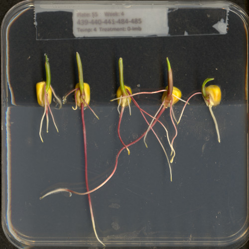
Now, let us zoom in and look at a small section of the label in the original, first in the uncompressed format:
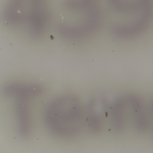
Here is the same area of the image, but in JPEG format. We used a fairly aggressive compression parameter to make the JPEG, in order to illustrate the problems you might encounter with the format.
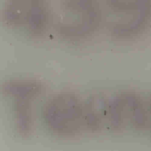
The JPEG image is of clearly inferior quality. It has less color variation and noticeable pixelation. Quality differences become even more marked when one examines the color histograms for each image. A histogram shows how often each color value appears in an image. The histograms for the uncompressed (left) and compressed (right) images are shown below:
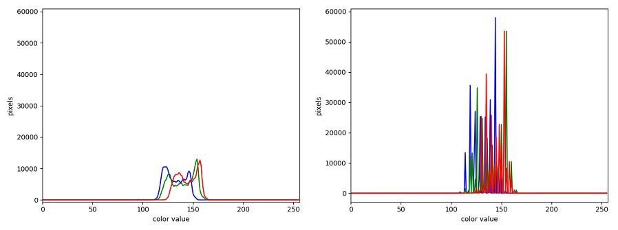
We we learn how to make histograms such as these later on in the workshop. The differences in the color histograms are even more apparent than in the images themselves; clearly the colors in the JPEG image are different from the uncompressed version.
If the quality settings for your JPEG images are high (and the compression rate therefore relatively low), the images may be of sufficient quality for your work. It all depends on how much quality you need, and what restrictions you have on image storage space. Another consideration may be where the images are stored. For example, if your images are stored in the cloud and therefore must be downloaded to your system before you use them, you may wish to use a compressed image format to speed up file transfer time.
TIFF
TIFF images are popular with publishers, graphics designers, and photographers. TIFF images can be uncompressed, or compressed using either lossless or lossy compression schemes, depending on the settings used, and so TIFF images seem to have the benefits of both the BMP and JPEG formats. The main disadvantage of TIFF images (other than the size of images in the uncompressed version of the format) is that they are not universally readable by image viewing and manipulation software.
Metadata
JPEG and TIFF images support the inclusion of metadata in images. Metadata is textual information that is contained within an image file. Metadata holds information about the image itself, such as when the image was captured, where it was captured, what type of camera was used and with what settings, etc. We normally don’t see this metadata when we view an image, but we can access it if we wish. For example, consider this image of a tree flowering in spring:
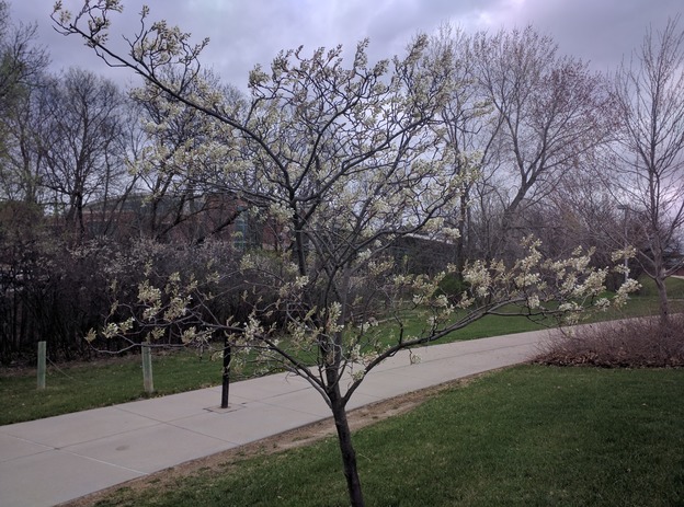
What metadata do you suppose this image contains? One way we can find out is by using ImageMagick, a public domain image processing program that is available for many different computing platforms. ImageMagick is installed on the virtual machine used for this workshop. To display the metadata for an image, we can execute the identify -verbose <file> command from the terminal. If we were to view the tree image metadata with ImageMagick, we would see this information, plus another 100 lines or so:
[Jpeg] Compression Type:	Baseline
[Jpeg] Data Precision:	8 bits
[Jpeg] Image Height:	463 pixels
[Jpeg] Image Width:	624 pixels
[Jpeg] Number of Components:	3
[Jpeg] Component 1:	Y component: Quantization table 0, Sampling factors 2 horiz/2 vert
[Jpeg] Component 2:	Cb component: Quantization table 1, Sampling factors 1 horiz/1 vert
[Jpeg] Component 3:	Cr component: Quantization table 1, Sampling factors 1 horiz/1 vert
[Jfif] Version:	1.1
[Jfif] Resolution Units:	inch
[Jfif] X Resolution:	72 dots
[Jfif] Y Resolution:	72 dots
[Exif SubIFD] Exposure Time:	657/1000000 sec
[Exif SubIFD] F-Number:	F2
[Exif SubIFD] Exposure Program:	Program normal
[Exif SubIFD] ISO Speed Ratings:	40
[Exif SubIFD] Exif Version:	2.20
[Exif SubIFD] Date/Time Original:	2017:04:10 12:04:06
[Exif SubIFD] Date/Time Digitized:	2017:04:10 12:04:06
[Exif SubIFD] Components Configuration:	YCbCr
[Exif SubIFD] Shutter Speed Value:	1/1520 sec
[Exif SubIFD] Aperture Value:	F2
[Exif SubIFD] Brightness Value:	8.89
[Exif SubIFD] Exposure Bias Value:	0 EV
[Exif SubIFD] Max Aperture Value:	F2
[Exif SubIFD] Subject Distance:	0.0 metres
[Exif SubIFD] Metering Mode:	Center weighted average
[Exif SubIFD] Flash:	Flash did not fire, auto
[Exif SubIFD] Focal Length:	3.82 mm
[Exif SubIFD] Sub-Sec Time:	025669
[Exif SubIFD] Sub-Sec Time Original:	025669
[Exif SubIFD] Sub-Sec Time Digitized:	025669
[Exif SubIFD] FlashPix Version:	1.00
[Exif SubIFD] Color Space:	sRGB
[Exif SubIFD] Exif Image Width:	4160 pixels
[Exif SubIFD] Exif Image Height:	3088 pixels
[Exif SubIFD] Sensing Method:	One-chip color area sensor
[Exif SubIFD] Scene Type:	Directly photographed image
[Exif SubIFD] Custom Rendered:	Custom process
[Exif SubIFD] Exposure Mode:	Auto exposure
[Exif SubIFD] White Balance Mode:	Auto white balance
[Exif SubIFD] Scene Capture Type:	Standard
[Exif SubIFD] Contrast:	None
[Exif SubIFD] Saturation:	None
[Exif SubIFD] Sharpness:	None
[Exif SubIFD] Subject Distance Range:	Unknown
[Exif SubIFD] Unknown tag (0xea1c):	[2060 bytes]
[Exif SubIFD] Unknown tag (0xea1d):	4264
[Exif IFD0] Unknown tag (0x0100):	4160
[Exif IFD0] Unknown tag (0x0101):	3088
[Exif IFD0] Image Description:	Flowering tree
[Exif IFD0] Make:	motorola
[Exif IFD0] Model:	Nexus 6
[Exif IFD0] Orientation:	Top, left side (Horizontal / normal)
[Exif IFD0] X Resolution:	72 dots per inch
[Exif IFD0] Y Resolution:	72 dots per inch
[Exif IFD0] Resolution Unit:	Inch
[Exif IFD0] Software:	HDR+ 1.0.126161355r
[Exif IFD0] Date/Time:	2017:04:10 12:04:06
[Exif IFD0] Artist:	Mark M. Meysenburg
[Exif IFD0] YCbCr Positioning:	Center of pixel array
[Exif IFD0] Unknown tag (0x4746):	5
[Exif IFD0] Unknown tag (0x4749):	99
[Exif IFD0] Windows XP Title:	Flowering tree
[Exif IFD0] Windows XP Author:	Mark M. Meysenburg
[Exif IFD0] Windows XP Subject:	Nature
[Exif IFD0] Unknown tag (0xea1c):	[2060 bytes]
[Interoperability] Interoperability Version:	1.00
[GPS] GPS Version ID:	2.200
[GPS] GPS Latitude Ref:	N
[GPS] GPS Latitude:	40.0° 37.0' 19.33999999999571"
[GPS] GPS Longitude Ref:	W
[GPS] GPS Longitude:	-96.0° 56.0' 46.74000000003048"
[GPS] GPS Altitude Ref:	Sea level
[GPS] GPS Altitude:	405 metres
[GPS] GPS Time-Stamp:	17:4:3 UTC
Reviewing the metadata, you can see things like the location where the image was taken, the make and model of the Android smartphone used to capture the image, the date and time when it was captured, and more. Two tags, containing the image description and the “artist,” were added manually. Depending on how you intend to use images, the metadata contained within the images may be important or useful to you. However, care must be taken when using our computer vision library, skimage, to write images. We will examine metadata a little more closely in the skimage Images episode.
Summary of image formats
The following table summarizes the characteristics of the BMP, JPEG, and TIFF image formats:
| Format | Compression | Metadata | Advantages | Disadvantages |
|---|---|---|---|---|
| BMP | None | None | Universally viewable, | Large file sizes |
| high quality | ||||
| JPEG | Lossy | Yes | Universally viewable, | Detail may be lost |
| smaller file size | ||||
| TIFF | None, lossy, | Yes | High quality or | Not universally viewable |
| or lossless | smaller file size |
Key Points
Digital images are represented as rectangular arrays of square pixels.
Digital images use a left-hand coordinate system, with the origin in the upper left corner, the x-axis running to the right, and the y-axis running down.
Most frequently, digital images use an additive RGB model, with eight bits for the red, green, and blue channels.
Lossless compression retains all the details in an image, but lossy compression results in loss of some of the original image detail.
BMP images are uncompressed, meaning they have high quality but also that their file sizes are large.
JPEG images use lossy compression, meaning that their file sizes are smaller, but image quality may suffer.
TIFF images can be uncompressed or compressed with lossy or lossless compression.
Depending on the camera or sensor, various useful pieces of information may be stored in an image file, in the image metadata.